Sharpe Ratio

Distribution of Maximal Sharpe, Truncated Normal

In a previous blog post we looked at a symmetric confidence intervals on the Signal-Noise ratio. That study was motivated by the "opportunistic strategy", wherein one observes the historical returns of an asset to determine whether to hold it long or short. Then, conditional on the sign of the trade, we were able to construct proper confidence intervals on the Signal-Noise ratio of the opportunistic strategy's returns.

I had hoped that one could generalize from the single asset opportunistic strategy to the case of $p$ assets, where one constructs the Markowitz portfolio based on observed returns. I have not had much luck finding that generalization. However, we can generalize the opportunistic strategy in a different way to what I call the "Winner Take All" strategy. Here one observes the historical returns of $p$ different assets, then chooses the one with the highest observed Sharpe ratio to hold long. (Let us hold off on an Opportunistic Winner Take All.)

Observe, however, this is just the problem of inferring the Signal Noise ratio (SNR) of the asset with the maximal Sharpe. We previously approached that problem using a Markowitz approximation, finding it somewhat lacking. That Markowitz approximation was an attempt to correct some deficiencies with what is apparently the state of the art in the field, Marcos Lopez de Prado's (now AQR's?) "Most Important Plot in All of Finance", which is a thin layer of Multiple Hypothesis Testing correction over the usual distribution of the Sharpe ratio. In a previous blog post, we found that Lopez de Prado's method would have lower than nominal type I rates as it ignored correlation of assets.

Moreover, a simple MHT correction will not, I think, deal very well with the case where there are great differences in the Signal Noise ratios of the assets. The 'stinker' assets with low SNR will simply spoil our inference, unlikely to have much influence on which asset shows the highest Sharpe ratio, and only causing us to increase our significance threshold.

With my superior googling skills I recently discovered a 2013 paper by Lee et al, titled Exact Post-Selection Inference, with Application to the Lasso. While aimed at the Lasso, this paper includes a procedure that essentially solves our problem, giving hypothesis tests or confidence intervals with nominal coverage on the asset with maximal Sharpe among a set of possibly correlated assets.

The Lee et al paper assumes one observes $p$-vector $$ y \sim \mathcal{N}\left(\mu,\Sigma\right). $$ Then conditional on $y$ falling in some polyhedron, $Ay \le b$, we wish to perform inference on $\nu^{\top}y$. In our case the polyhedron will be the union of all polyhedra with the same maximal element of $y$ as we observed. That is, assume that we have reordered the elements of $y$ such that $y_1$ is the largest element. Then $A$ will be a column of negative ones, cbinded to the $p-1$ identity matrix, and $b$ will be a $p-1$ vector of zeros. The test is defined on $\nu=e_1$ the vector with a single one in the first element and zero otherwise.

Their method works by decomposing the condition $Ay \le b$ into a condition on $\nu^{\top}y$ and a condition on some $z$ which is normal but independent of $\nu^{\top}y$. You can think of this as kind of inverting the transform by $A$. After this transform, the value of $\nu^{\top}y$ is restricted to a line segment, so we need only perform inference on a truncated normal.

The code to implement this is fairly straightforward, and given below. The procedure to compute the quantile function, which we will need to compute confidence intervals, is a bit trickier, due to numerical issues. We give a hacky version below.

# Lee et. al eqn (5.8)
F_fnc <- function(x,a,b,mu=0,sigmasq=1) {
  sigma <- sqrt(sigmasq)
  phis <- pnorm((c(x,a,b)-mu)/sigma)
  (phis[1] - phis[2]) / (phis[3] - phis[2])
}
# Lee eqns (5.4), (5.5), (5.6)
Vfuncs <- function(z,A,b,ccc) {
  Az <- A %*% z
  Ac <- A %*% ccc
  bres <- b - Az
  brat <- bres
  brat[Ac!=0] <- brat[Ac!=0] / Ac[Ac!=0]
  Vminus <- max(brat[Ac < 0])
  Vplus  <- min(brat[Ac > 0])
  Vzero  <- min(bres[Ac == 0])
  list(Vminus=Vminus,Vplus=Vplus,Vzero=Vzero)
}
# Lee et. al eqn (5.9)
ptn <- function(y,A,b,nu,mu,Sigma,numu=as.numeric(t(nu) %*% mu)) {
  Signu <- Sigma %*% nu
  nuSnu <- as.numeric(t(nu) %*% Signu)
  ccc <- Signu / nuSnu  # eqn (5.3)
  nuy <- as.numeric(t(nu) %*% y)
  zzz <- y - ccc * nuy  # eqn (5.2)
  Vfs <- Vfuncs(zzz,A,b,ccc)
  F_fnc(x=nuy,a=Vfs$Vminus,b=Vfs$Vplus,mu=numu,sigmasq=nuSnu)
}
# invert the ptn function to find nu'mu at a given pval.
citn <- function(p,y,A,b,nu,Sigma) { 
  Signu <- Sigma %*% nu
  nuSnu <- as.numeric(t(nu) %*% Signu)
  ccc <- Signu / nuSnu  # eqn (5.3)
  nuy <- as.numeric(t(nu) %*% y)
  zzz <- y - ccc * nuy  # eqn (5.2)
  Vfs <- Vfuncs(zzz,A,b,ccc)

  # you want this, but there are numerical issues: 
  #f <- function(numu) { F_fnc(x=nuy,a=Vfs$Vminus,b=Vfs$Vplus,mu=numu,sigmasq=nuSnu) - p } 
  sigma <- sqrt(nuSnu)
  f <- function(numu) { 
    phis <- pnorm((c(nuy,Vfs$Vminus,Vfs$Vplus)-numu)/sigma)
    #(phis[1] - phis[2]) - p * (phis[3] - phis[2])
    phis[1] - (1-p) * phis[2] - p * phis[3]
  }
  # this fails sometimes, so find a better interval
  intvl <- c(-1,1)  # a hack.
  # this is very unfortunate
    trypnts <- seq(from=min(y),to=max(y),length.out=31)
    ys <- sapply(trypnts,f)
    dsy <- diff(sign(ys))
    if (any(dsy < 0)) {
      widx <- which(dsy < 0)
      intvl <- trypnts[widx + c(0,1)]
    } else {
      maby <- 2 * (0.1 + max(abs(y)))
      trypnts <- seq(from=-maby,to=maby,length.out=31)
      ys <- sapply(trypnts,f)
      dsy <- diff(sign(ys))
      if (any(dsy < 0)) {
        widx <- which(dsy < 0)
        intvl <- trypnts[widx + c(0,1)]
      }
    }
  uniroot(f=f,interval=intvl,extendInt='yes')$root
}

Testing on normal data

Here we test the code above on the problem considered in Theorem 5.2 of Lee et al. That is, we draw $y \sim \mathcal{N}\left(\mu,\Sigma\right)$, then observe the value of $F$ given in Theorem 5.2 when we plug in the actual population values of $\mu$ and $\Sigma$. This is several steps removed from our problem of inference on the SNR, but it is best to pause and make sure the implementation is correct first.

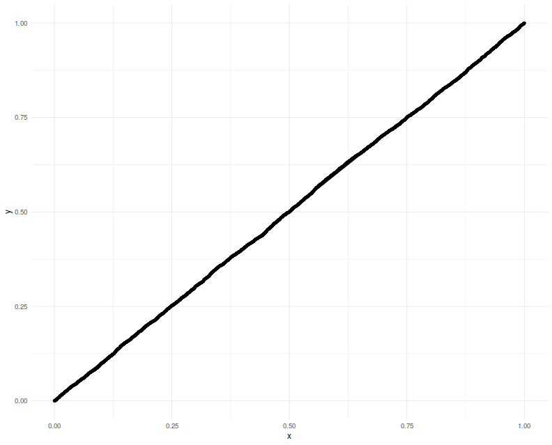
We perform 5000 simulations, letting $p=20$, then creating a random $\mu$ and $\Sigma$, drawing a single $y$, observing which element is the maximum, creating $A, b, \nu$, then computing the $F$ function, resulting in a $p$-value which should be uniform. We Q-Q plot those empirical $p$-values against a uniform law, finding them on the $y=x$ line.

gram <- function(x) { t(x) %*% x }
rWish <- function(n,p=n,Sigma=diag(p)) { 
  require(mvtnorm)
  gram(rmvnorm(p,sigma=Sigma))
}
nsim <- 5000
p <- 20
A1 <- cbind(-1,diag(p-1))
set.seed(1234)
pvals <- replicate(nsim,{
  mu <- rnorm(p)
  Sigma <- rWish(n=2*p+5,p=p)
  y <- t(rmvnorm(1,mean=mu,sigma=Sigma) )
  # collect the maximum, so reorder the A above
  yord <- order(y,decreasing=TRUE)
  revo <- seq_len(p)
  revo[yord] <- revo

  A <- A1[,revo]
  nu <- rep(0,p)
  nu[yord[1]] <- 1
  b <- rep(0,p-1)
  foo <- ptn(y=y,A=A,b=b,nu=nu,mu=mu,Sigma=Sigma)
})
# plot them:
library(dplyr)
library(ggplot2)
ph <- data_frame(pvals=pvals) %>%   
  ggplot(aes(sample=pvals)) + 
  geom_qq(distribution=stats::qunif) +
  geom_qq_line(distribution=stats::qunif) 
print(ph)

Now we attempt to use the confidence interval code. We construct a one-sided 95% confidence interval, and check how often it is violated by the $\mu$ of the element which shows the highest $y$. We will find that the empirical rate of violations of our confidence interval is indeed around 5%:

nsim <- 5000
p <- 20
A1 <- cbind(-1,diag(p-1))
set.seed(1234)
tgtval <- 0.95
viols <- replicate(nsim,{
  mu <- rnorm(p)
  Sigma <- rWish(n=2*p+5,p=p)
  y <- t(rmvnorm(1,mean=mu,sigma=Sigma) )
  # collect the maximum, so reorder the A above
  yord <- order(y,decreasing=TRUE)
  revo <- seq_len(p)
  revo[yord] <- revo

  A <- A1[,revo]
  nu <- rep(0,p)
  nu[yord[1]] <- 1
  b <- rep(0,p-1)
  # mu is unknown to this guy
  foo <- citn(p=tgtval,y=y,A=A,b=b,nu=nu,Sigma=Sigma)
  violated <- mu[yord[1]] < foo
})
print(sprintf('%.2f%%',100*mean(viols)))

[1] "5.04%"

Testing on the Sharpe ratio

To use this machinery to perform inference on the SNR, we can either port the results to the multivariate $t$-distribution, which seems unlikely because uncorrelated marginals of a multivariate $t$ are not independent. Instead we lean on the normal approximation to the vector of Sharpe ratios. If the $p$-vector $x$ is normal with correlation matrix $R$, then $$ \hat{\zeta}\approx\mathcal{N}\left(\zeta,\frac{1}{n}\left( R + \frac{1}{2}\operatorname{Diag}\left(\zeta\right)\left(R \odot R\right)\operatorname{Diag}\left(\zeta\right) \right)\right), $$ where $\hat{\zeta}$ is the $p$-vector of Sharpe ratios computed by observing $n$ independent draws of $x$, and $\zeta$ is the $p$-vector of Signal Noise ratios. Note how this generalizes the 'Lo' form of the standard error of a scalar Sharpe ratio, viz $\sqrt{(1 + \zeta^2/2)/n}$.

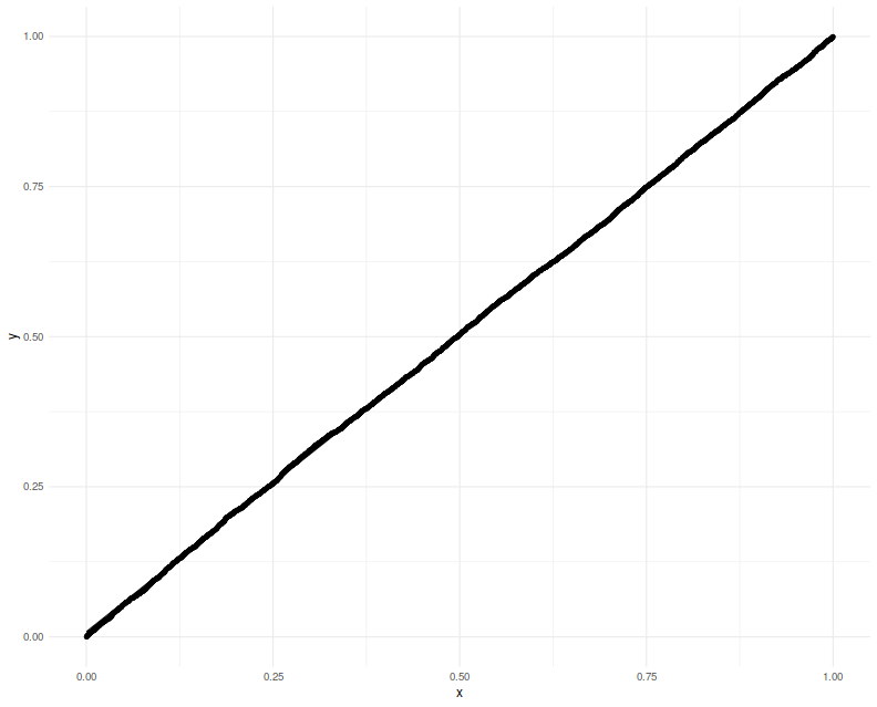
Here we will check the uniformity of $p$ values resulting from using this normal approximation. This is closer to the actual inference we want to do, except we will cheat by using the actual $R$ and $\zeta$ to construct what is essentially the $\Sigma$ to Lee's formulation. We will set $p=20$ and draw 3 years of daily data. Again we plot the putative $p$-values against uniformity and find a good match.

# let's test it!
nsim <- 5000
p <- 20
ndays <- 3 * 252
A1 <- cbind(-1,diag(p-1))
set.seed(4321)

pvals <- replicate(nsim,{
  # population values here
  mu <- rnorm(p)
  Sigma <- rWish(n=2*p+5,p=p)
  RRR <- cov2cor(Sigma)
  zeta <- mu /sqrt(diag(Sigma))

  Xrets <- rmvnorm(ndays,mean=mu,sigma=Sigma) 
  srs <- colMeans(Xrets) / apply(Xrets,2,FUN=sd)

  y <- srs
  mymu <- zeta
  mySigma <- (1/ndays) * (RRR + (1/2) * diag(zeta) %*% (RRR * RRR) %*% diag(zeta))

  # collect the maximum, so reorder the A above
  yord <- order(y,decreasing=TRUE)
  revo <- seq_len(p)
  revo[yord] <- revo

  A <- A1[,revo]
  nu <- rep(0,p)
  nu[yord[1]] <- 1
  b <- rep(0,p-1)

  foo <- ptn(y=y,A=A,b=b,nu=nu,mu=mymu,Sigma=mySigma)
})
# plot them:
library(dplyr)
library(ggplot2)
ph <- data_frame(pvals=pvals) %>%   
  ggplot(aes(sample=pvals)) + 
  geom_qq(distribution=stats::qunif) +
  geom_qq_line(distribution=stats::qunif) 
print(ph)

Lastly we make one more modification, filling in sample estimates for $\zeta$ and $R$ into the computation of the covariance. We compute one-sided 95% confidence intervals, and check how the empirical rate of violations. We find the rate to be around 5%.

nsim <- 5000
p <- 20
ndays <- 3 * 252
A1 <- cbind(-1,diag(p-1))
set.seed(9873)  # 5678 gives exactly 250 / 5000, which is eerie

tgtval <- 0.95
viols <- replicate(nsim,{
  # population values here
  mu <- rnorm(p)
  Sigma <- rWish(n=2*p+5,p=p)
  RRR <- cov2cor(Sigma)
  zeta <- mu /sqrt(diag(Sigma))

  Xrets <- rmvnorm(ndays,mean=mu,sigma=Sigma) 
  srs <- colMeans(Xrets) / apply(Xrets,2,FUN=sd)
  Sighat <- cov(Xrets)
  Rhat <- cov2cor(Sighat)

  y <- srs
  # now use the sample approximations. 
  # you can compute this from the observed information.
  mySigma <- (1/ndays) * (Rhat + (1/2) * diag(srs) %*% (Rhat * Rhat) %*% diag(srs))

  # collect the maximum, so reorder the A above
  yord <- order(y,decreasing=TRUE)
  revo <- seq_len(p)
  revo[yord] <- revo

  A <- A1[,revo]
  nu <- rep(0,p)
  nu[yord[1]] <- 1
  b <- rep(0,p-1)

  # mu is unknown to this guy
  foo <- citn(p=tgtval,y=y,A=A,b=b,nu=nu,Sigma=mySigma)
  violated <- zeta[yord[1]] < foo
})
print(sprintf('%.2f%%',100*mean(viols)))

[1] "5.14%"

Putting it together

Lee's method appears to give nominal coverage for hypothesis tests and confidence intervals on the SNR of the asset with maximal Sharpe. In principle it should not be affected by correlation of the assets or by large differences in the SNRs of the assets. It should be applicable in the $p > n$ case, as we are not inverting the covariance matrix. On the negative side, requiring one estimate the correlation of assets for the computation will not scale with large $p$.

We are guardedly optimistic that this method is not adversely affected by the normal approximation of the Sharpe ratio, although it would be ill-advised to use it for the case of small samples until more study is performed. Moreover the quantile function we hacked together here should be improved for stability and accuracy.

Symmetric Confidence Intervals, and Choosing Sides

Consider the problem of computing confidence intervals on the Signal-Noise ratio, which is the population quantity $\zeta = \mu/\sigma$, based on the observed Sharpe ratio $\hat{\zeta} = \hat{\mu}/\hat{\sigma}$. If returns are Gaussian, one can compute 'exact' confidence intervals by inverting the CDF of the non-central $t$ distribution with respect to its parameter. Typically instead one often uses an approximate standard error, using either the formula published by Johnson & Welch (and much later by Andrew Lo), or one using higher order moments given by Mertens, then constructs Wald-test confidence intervals.

Using standard errors yields symmetric intervals of the form $$ \hat{\zeta} \pm z_{\alpha/2} s, $$ where $s$ is the approximate standard error, and $z_{\alpha/2}$ is the normal $\alpha/2$ quantile. As typically constructed, the 'exact' confidence intervals based on the non-central $t$ distributionare not symmetric in general, but are very close, and can be made symmetric. The symmetry condition can be expressed as $$ \mathcal{P}\left(|\zeta - \hat{\zeta}| \ge c\right) = \alpha, $$ where $c$ is some constant.

Picking sides

Usually I think of the Sharpe ratio as a tool to answer the question: Should I invest a predetermined amount of capital (long) in this asset? The Sharpe ratio can be used to construct confidence intervals on the Signal-Noise ratio to help answer that question.

Pretend instead that you are more opportunistic: instead of considering a predetermined side to the trade, you will observe historical returns of the asset. Then if the Sharpe ratio is positive, you will consider investing in the asset, and if the Sharpe is negative, you will consider shorting the asset. Can we rely on our standard confidence intervals now? After all, we are now trying to perform inference on $\operatorname{sign}\left(\hat{\zeta}\right) \zeta$, which is not a population quantity. Rather it mixes up the population Signal-Noise ratio with information from the observed sample (the sign of the Sharpe). (Because of this mixing of a population quantity with information from the sample, real statisticians get a bit indignant when you try to call this a "confidence interval". So don't do that.)

It turns out that you can easily adapt the symmetric confidence intervals to this problem. Because you can multiply the inside of $\left|\zeta - \hat{\zeta}\right|$ by $\pm 1$ without affecting the absolute value, we have $$ \left|\zeta - \hat{\zeta}\right| \ge c \Leftrightarrow \left| \operatorname{sign}\left(\hat{\zeta}\right) \zeta - \left|\hat{\zeta}\right|\right| \ge c. $$ Thus $$ \left|\hat{\zeta}\right| \pm z_{\alpha/2} s $$ are $1-\alpha$ confidence intervals on $\operatorname{sign}\left(\hat{\zeta}\right) \zeta$.

Although the type I error rate is maintained, the 'violations' of the confidence interval can be asymmetric. When the Signal Noise ratio is large (in absolute value), type I errors tend to occur on both sides of the confidence interval equally, because the Sharpe is usually the same sign as the Signal-Noise ratio. When the Signal-Noise ratio is near zero, however, typically the type I errors occur only on the lower side. (This must be the case when the Signal-Noise ratio is exactly zero.) Of course, since the Signal-Noise ratio is the unknown population parameter, you do not know which situation you are in, although you have some hints from the observed Sharpe ratio.

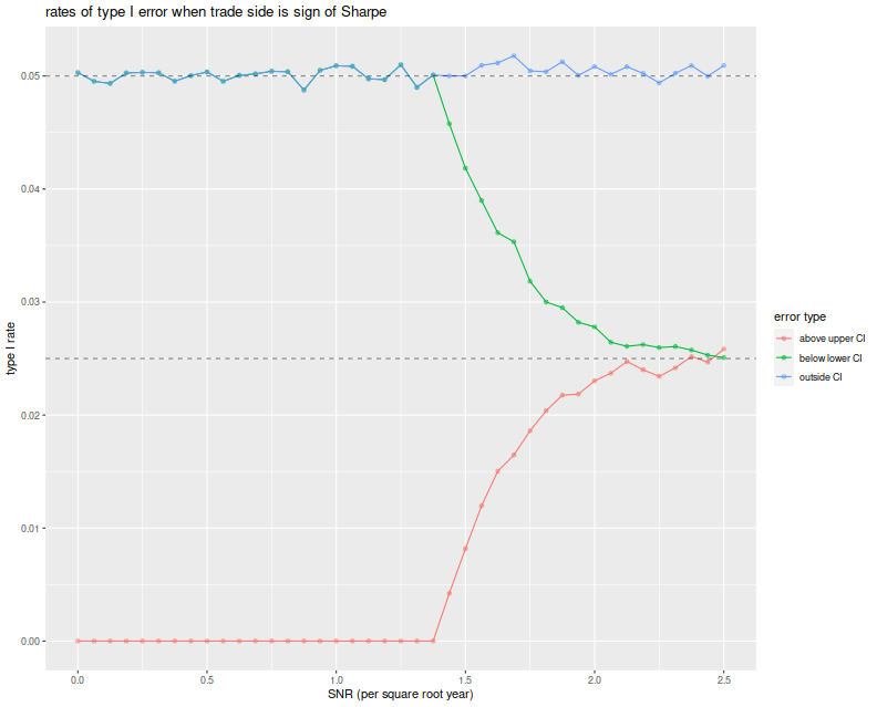
Before moving on, here we test the symmetric confidence intervals. We vary the Signal Noise ratio from 0 to 2.5 in 'annual units', draw two years of daily normal returns with that Signal-Noise ratio, pick a side of the trade based on the sign of the Sharpe ratio, then build symmetric confidence intervals using the standard error estimator $\sqrt{(1 + \hat{\zeta}^2/2)/n}$. We build the 95% confidence intervals, then note any breaches of the upper and lower confidence bounds. We repeat this 10000 times for each choice of SNR.

We then plot the type I rate for the lower bound of the CI, the upper bound and the total type I rate, versus the Signal Noise ratio. We see that the total empirical type I rate is very near the nominal rate of 5%, and this is entirely attributable to violations of the lower bound up until a Signal Noise ratio of around 1.4 per square root year. At around 2.5 per square root year, the type I errors are observed in equal proportion on both sides of the CI.

suppressMessages({
  library(dplyr)
  library(tidyr)
  library(future.apply)
})
# run one simulation of normal returns and CI violations
onesim <- function(n,pzeta,zalpha=qnorm(0.025)) {
    x <- rnorm(n,mean=pzeta,sd=1)
    sr <- mean(x) / sd(x)
    se <- sqrt((1+0.5*sr^2)/n)
    cis <- abs(sr) + se * abs(zalpha) * c(-1,1)
    pquant <- sign(sr) * pzeta
    violations <- c(pquant < cis[1],pquant > cis[2])
}
# do a bunch of sims, then sum the violations of low and high;
repsim <- function(nrep,n,pzeta,zalpha) {
  jumble <- replicate(nrep,onesim(n=n,pzeta=pzeta,zalpha=zalpha))
  retv <- t(jumble)
  colnames(retv) <- c('nlo','nhi')
  retv <- as.data.frame(retv) %>%
        summarize_all(.funs=sum)
    retv$nrep <- nrep
    invisible(retv)
}
manysim <- function(nrep,n,pzeta,zalpha,nnodes=7) {
  if (nrep > 2*nnodes) {
        plan(multisession, workers = 7)  
    # do in parallel.
    nper <- table(1 + ((0:(nrep-1) %% nnodes))) 
    retv <- future_lapply(nper,function(aper) repsim(nrep=aper,n=n,pzeta=pzeta,zalpha=zalpha)) %>%
      bind_rows() %>%
            summarize_all(.funs=sum) 
        plan(sequential)
  } else {
    retv <- repsim(nrep=nrep,n=n,pzeta=pzeta,zalpha=zalpha)
  }
    # turn sums into means
    retv %>%
        mutate(vlo=nlo/nrep,vhi=nhi/nrep) %>%
        dplyr::select(vlo,vhi)
}

# run a bunch
ope <- 252
nyr <- 2
alpha <- 0.05

# simulation params
params <- data_frame(zetayr=seq(0,2.5,by=0.0625)) %>%
    mutate(pzeta=zetayr/sqrt(ope)) %>%
    mutate(n=round(ope*nyr))

# run a bunch
nrep <- 100000
set.seed(4321)
system.time({
results <- params %>%
  group_by(zetayr,pzeta,n) %>%
    summarize(sims=list(manysim(nrep=nrep,nnodes=7,
                                pzeta=pzeta,n=n,zalpha=qnorm(alpha/2)))) %>%
  ungroup() %>%
  tidyr::unnest() 
})

suppressMessages({
  library(dplyr)
  library(tidyr)
  library(ggplot2)
})
ph <- results %>%
    mutate(vtot=vlo+vhi) %>%
    gather(key=series,value=violations,vlo,vhi,vtot) %>%
    mutate(series=case_when(.$series=='vlo' ~ 'below lower CI',
                                                    .$series=='vhi' ~ 'above upper CI',
                                                    .$series=='vtot' ~ 'outside CI',
                                                    TRUE ~ 'error')) %>%
    ggplot(aes(zetayr, violations, colour=series)) + 
    geom_line() + geom_point(alpha=0.5) + 
    geom_hline(yintercept=c(alpha/2,alpha),linetype=2,alpha=0.5) +
    labs(x='SNR (per square root year)',y='type I rate',
             color='error type',title='Rates of type I error when trade side is sign of Sharpe')
print(ph)

A Bayesian Donut?

Of course, this strategy seems a bit unrealistic: what's the point of constructing confidence intervals if you are going to trade the asset no matter what the evidence? Instead, consider a fund manager whose trading strategies are all above average: she/he observes the Sharpe ratio of a backtest, then only trades a strategy if $|\hat{\zeta}| \ge c$ for some sufficiently large $c$, and picks a side based on $\operatorname{sign}\left(\hat{\zeta}\right)$. This is a 'donut'.

Conditional on observing $|\hat{\zeta}| \ge c$, can one construct a reliable confidence interval on $\operatorname{sign}\left(\hat{\zeta}\right) \zeta$? Perhaps our fund manager thinks there is no point in doing so if $c$ is sufficiently large. I think to do so you have to make some assumptions about the distribution of $\zeta$ and rely on Baye's law. We did not say what would happen if the junior quant at this shop developed a strategy where $|\hat{\zeta}| < c$, but presumably the junior quants were told to keep working until they beat the magic threshold. If the junior quants only produce strategies with small $\zeta$, one suspects that the $c$ threshold does very little to reject bad strategies, rather it just slows down their deployment. (In response the quants will surely beef up their backtesting infrastructure, or invent automatic strategy generation.)

Generalizing to higher dimensions

The real interesting question is what this looks like in higher dimensions. Now one observes $p$ assets, and is to construct a portfolio on those assets. Can we construct good confidence intervals on the Sharpe ratio of the chosen portfolio? In this setting we have many more possible choices, so a general purpose analysis seems unlikely. However, if we restrict ourselves to the Markowitz portfolio, I suspect some progress can be made. (Although I have been very slow to make it!) I hope to purse this in a followup blog post.

A Sharper Sharpe: Its Biased.

Note: This blog post previously analyzed Damien Challet's 'Sharper estimator' of the Signal-Noise Ratio. In a series of blog posts, I had found that the implementation of this estimator appeared to be biased, giving perhaps illusory gains in efficiency. I had noted in this post that I contacted Challet to present my concerns about his code. Since the time I wrote that post, Challet updated his sharpeRratio, package to version 1.2. We will perform an investigation of the fixed drawdown estimator, and link to it here.

Distribution of Maximal Sharpe, the Markowitz Approximation

In a previous blog post we looked at a statistical test for overfitting of trading strategies proposed by Lopez de Prado, which essentially uses a $t$-test threshold on the maximal Sharpe of backtested returns based on assumed independence of the returns. (Actually it is not clear if Lopez de Prado suggests a $t$-test or relies on approximate normality of the $t$, but they are close enough.) In that blog post, we found that in the presence of mutual positive correlation of the strategies, the test would be somewhat conservative. It is hard to say just how conservative the test would be without making some assumptions about the situations in which it would be used.

This is a trivial point, but needs to be mentioned: to create a useful test of strategy overfitting, one should consider how strategies are developed and overfit. There are numerous ways that trading strategies are, or could be developed. I will enumerate some here, roughly in order of decreasing methodological purity:

1. Alice the Quant goes into the desert on a Vision Quest. She emerges three days later with a fully formed trading idea, and backtests it a single time to satisfy the investment committee. The strategy is traded unconditional on the results of that backtest.

2. Bob the Quant develops a black box that generates, on demand, a quantitative trading strategy, and performs a backtest on that strategy to produce an unbiased estimate of the historical performance of the strategy. All strategies are produced de novo, without any relation to any other strategy ever developed, and all have independent returns. The black box can be queried ad infinitum. (This is essentially Lopez de Prado's assumed mode of development.)

3. The same as above, but the strategies possibly have correlated returns, or were possibly seeded by published anomalies or trading ideas.

4. Carole the Quant produces a single new trading idea, in a white box, that is parametrized by a number of free parameters. The strategy is backtested on many settings of those parameters, which are chosen by some kind of design, and the settings which produce the maximal Sharpe are selected.

5. The same as above, except the parameters are optimized based on backtested Sharpe using some kind of hill-climbing heuristic or an optimizer.

6. The same as above, except the trading strategy was generally known and possibly overfit by other parties prior to publication as "an anomaly".

7. Doug the Quant develops a gray box trading idea, adding and removing parameters while backtesting the strategy and debugging the code, mixing machine and human heuristics, and leaving no record of the entire process.

8. A small group of Quants separately develop a bunch of trading strategies, using common data and tools, but otherwise independently hillclimb the in-sample Sharpe, adding and removing parameters, each backtesting countless unknown numbers of times, all in competition to have money allocated to their strategies.

9. The same, except the fund needs to have a 'good quarter', otherwise investors will pull their money, and they really mean it this time.

The first development mode is intentionally ludicrous. (In fact, these modes are also roughly ordered by increasing realism.) It is the only development model that might result in underfitting. The division between the second and third modes is loosely quantifiable by the mutual correlation among strategies, as considered in the previous blog post. But it is not at all clear how to approach the remaining development modes with the maximal Sharpe statistic. Perhaps a "number of pseudo-independent backtests" could be estimated and then used with the proposed test, but one cannot say how this would work with in-sample optimization, or the diversification benefit of looking in multidimensional parameter space.

The Markowitz Approximation

Perhaps the maximal Sharpe test can be salvaged, but I come to bury Caesar, not to resuscitate him. Some years ago, I developed a test for overfitting based on an approximate portfolio problem. I am ashamed to say, however, that while writing this blog post I have discovered that this approximation is not as accurate as I had remembered! It is interesting enough to present, I think, warts and all.

Suppose you could observe the time series of backtested returns from all the backtests considered. By 'all', I want to be very inclusive if the parameters were somehow optimized by some closed form equation, say. Let $Y$ be the $n \times k$ matrix of returns, with each row a date, and each column one of the backtests. We suppose we have selected the strategy which maximizes Sharpe, which corresponds to picking the column of $Y$ with the largest Sharpe.

Now perform some kind of dimensionality reduction on the matrix $Y$ to arrive at $$ Y \approx X W, $$ where $X$ is an $n \times l$ matrix, and $W$ is an $l \times k$ matrix, and where $l \ll k$. The columns of $X$ approximately span the columns of $Y$. Picking the strategy with maximal Sharpe now approximately corresponds to picking a column of $W$ that has the highest Sharpe when multiplied by $X$. That is, our original overfitting approximately corresponded to the optimization problem $$ \max_{w \in W} \operatorname{Sharpe}\left(X w\right). $$

The unconstrained version of this optimization problem is solved by the Markowitz portfolio. Moreover, if the returns $X$ are multivariate normal with independent rows, then the distribution of the (squared) Sharpe of the Markowitz portfolio is known, both under the null hypothesis (columns of $X$ are all zero mean), and the alternative (the maximal achievable population Sharpe is non-zero), via Hotelling's $T^2$ statistic.

If $\hat{\zeta}$ is the (in-sample) Sharpe of the (in-sample) Markowitz portfolio on $X$, assumed i.i.d. Normal, then $$ \frac{(n-l) \hat{\zeta}^2}{l (n - 1)} $$ follows an F distribution with $l$ and $n-l$ degrees of freedom. I wrote the psropt and qsropt functions in SharpeR to compute the CDF and quantile of the maximal in-sample Sharpe to support this kind of analysis.

I should note there are a few problems with this approximation:

1. There is no strong theoretical basis for this approximation: we do not have a model for how correlated returns should arise for a particular population, nor what the dimension $l$ should be, nor what to expect under the alternative, when the true optimal strategy has positive Sharpe. (I suspect that posing overfit of backtests as a Gaussian Process might be fruitful.)

2. We have to estimate the dimensionality, $l$, which is about as odious as estimating the number of 'pseudo-observations' in the maximal Sharpe test. I had originally suspected that $l$ would be 'obvious' from the application, but this is not apparently so.

3. Although the returns may live nearly in an $l$ dimensional subspace, we might have have selected a suboptimal combination of them in our overfitting process. This would be of no consequence if the $l$ were accurately estimated, but it will stymie our testing of the approximation.

Despite these problems, let us press on.

An example: a two window Moving Average Crossover

While writing this blog post, I went looking for examples of 'classical' technical strategies which would be ripe for overfitting (and which I could easily simulate under the null hypothesis). I was surprised to find that freely available material on Technical Analysis was even worse than I could imagine. Nowhere among the annotated plots with silly drawings could I find a concrete description of a trading strategy, possibly with free parameters to be fit to the data. Rather than wade through that swamp any longer, I went with an old classic, the Moving Average Crossover.

The idea is simple: compute two moving averages of the price series with different windows. When one is greater than the other, hold the asset long, otherwise hold it short. The choice of two windows must be overfit by the quant. Here I perform that experiment, but under the null hypothesis, with zero mean simulated returns generated independently of each other. Any realization of this strategy, with any choice of the windows, will have zero mean returns and thus zero Sharpe.

First I collect 'backtests' (sans any trading costs) of two window MAC for a single realization of returns where the two windows were allowed to vary from 2 to around 1000. The backtest period is 5 years of daily data. I compute the singular value decomposition of the returns, then present a scree plot of the singular values.

suppressMessages({
  library(dplyr)
  library(fromo)
    library(svdvis)
    library(ggplot2)
})
# return time series of *all* backtests
backtests <- function(windows,rel_rets) {
    nwin <- length(windows)
    nc <- choose(nwin,2) 

    fwd_rets <- dplyr::lead(rel_rets,1)
    # log returns
    log_rets <- log(1 + rel_rets)
    # price series
    psers <- exp(cumsum(log_rets))
    avgs <- lapply(windows,fromo::running_mean,v=psers)

    X <- matrix(0,nrow=length(rel_rets),ncol=2*nc)

    idx <- 1
    for (iii in 1:(nwin-1)) {
        for (jjj in (iii+1):nwin) {
            position <- sign(avgs[[iii]] - avgs[[jjj]])
            myrets <- position * fwd_rets
            X[,idx] <- myrets
            X[,idx+1] <- -myrets
            idx <- idx + 1
        }
    }
    # trim the last row, which has the last NA
    X <- X[-nrow(X),]
    X
}
geomseq <- function(from=1,to=1,by=(to/from)^(1/(length.out-1)),length.out=NULL) {
    if (missing(length.out)) { 
        lseq <- seq(log(from),log(to),by=log(by)) 
    } else {
        lseq <- seq(log(from),log(to),by=log(by),length.out=length.out)
    }
    exp(lseq)
}

# which windows to test
windows <- unique(ceiling(geomseq(2,1000,by=1.15))) 
nobs <- ceiling(3 * 252)
maxwin <- max(windows)
rel_rets <- rnorm(maxwin + 10 + nobs,mean=0,sd=0.01)

XX <- backtests(windows,rel_rets)
# grab the last nobs rows
XX <- XX[(nrow(XX)-nobs+1):(nrow(XX)),]

# perform svd
blah <- svd(x=XX,nu=11,nv=11)
# look at it
ph <- svdvis::svd.scree(blah) +
    labs(x='Singular Vectors',y='Percent Variance Explained') 
print(ph)

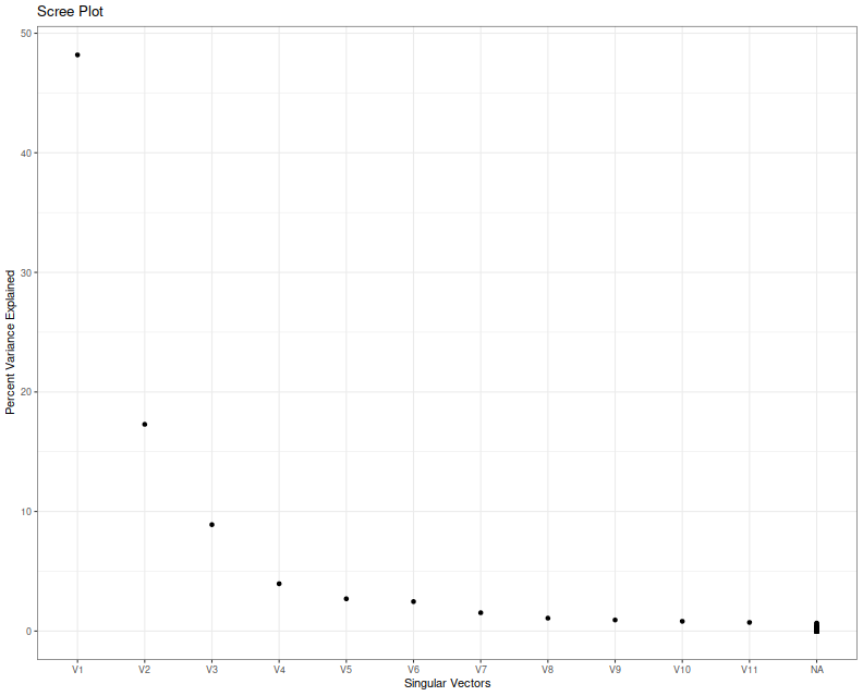
I think we can agree that nobody knows how to interpret a scree plot. However, in this case a large proportion of the explained variance seems to encoded in the first two eigenvalues, which is consistent with my a priori guess that $l=2$ in this case because of the two free parameters.

Next I simulate overfitting, performing that same experiment, but picking the largest in-sample Sharpe ratio. I create a series of independent zero mean returns, then backtest a bunch of MAC strategies, and save the maximal Sharpe over a 3 year window of daily data. I repeat this experiment ten thousand times, and then look at the distribution of that maximal Sharpe.

suppressMessages({
  library(dplyr)
  library(tidyr)
  library(tibble)
  library(SharpeR)
  library(future.apply)
  library(ggplot2)
})
ope <- 252

geomseq <- function(from=1,to=1,by=(to/from)^(1/(length.out-1)),length.out=NULL) {
    if (missing(length.out)) { 
        lseq <- seq(log(from),log(to),by=log(by)) 
    } else {
        lseq <- seq(log(from),log(to),by=log(by),length.out=length.out)
    }
    exp(lseq)
}
# one simulation. returns maximal Sharpe
onesim <- function(windows,n=1000) {
    maxwin <- max(windows)
    rel_rets <- rnorm(maxwin + 10 + n,mean=0,sd=0.01)
    fwd_rets <- dplyr::lead(rel_rets,1)
    # log returns
    log_rets <- log(1 + rel_rets)
    # price series
    psers <- exp(cumsum(log_rets))
    avgs <- lapply(windows,fromo::running_mean,v=psers)

    nwin <- length(windows)
    maxsr <- 0

    for (iii in 1:(nwin-1)) {
        for (jjj in (iii+1):nwin) {
            position <- sign(avgs[[iii]] - avgs[[jjj]])
            myrets <- position * fwd_rets
            # compute Sharpe on some part of this
            compon <- myrets[(length(myrets)-n):(length(myrets)-1)]
            thissr <- SharpeR::as.sr(compon,ope=ope)$sr
            # we are implicitly testing both combinations of long and short here,
            # so we take the absolute Sharpe, since we will always overfit to
            # the better of the two:
            maxsr <- max(maxsr,abs(thissr))
        }
    }
    maxsr
}

windows <- unique(ceiling(geomseq(2,1000,by=1.15))) 
nobs <- ceiling(3 * 252)
nrep <- 10000
plan(multicore)
set.seed(1234)
system.time({
    simvals <- future_replicate(nrep,onesim(windows,n=nobs))
})

    user   system  elapsed 
1227.959    4.398  307.299 

Here I plot the empirical quantiles of the maximal (annualized) Sharpe versus theoretical quantiles under the Markowitz approximation, assuming $l=2$. I also plot the $y=x$ lines, and horizontal and vertical lines at the nominal upper $0.05$ cutoff based on the Markowitz approximation.

# plot max value vs quantile:
library(ggplot2)
apxdf <- 2.0
ph <- data.frame(simvals=simvals) %>%
    ggplot(aes(sample=simvals)) + 
    geom_vline(xintercept=SharpeR::qsropt(0.95,df1=apxdf,df2=nobs,zeta.s=0,ope=ope),linetype=3) +
    geom_hline(yintercept=SharpeR::qsropt(0.95,df1=apxdf,df2=nobs,zeta.s=0,ope=ope),linetype=3) +
    stat_qq(distribution=SharpeR::qsropt,dparams=list(df1=apxdf,df2=nobs,zeta.s=0,ope=ope)) +
    geom_abline(intercept=0,slope=1,linetype=2) + 
    labs(title='empirical quantiles of maximal Sharpe versus Markowitz Approximation',
             x='theoretical quantile',y='empirical quantile (Sharpe in annual units)')
print(ph)

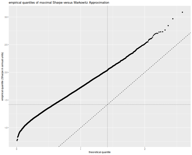
This approximation is clearly no good. The empirical rate of type I errors at the $0.05$ level is around 60%, and the Q-Q line is just off. I must admit that when I previously looked at this approximation (and in the vignette for SharpeR!) I used the qqline function in base R, which fits a line based on the first and third quartile of the empirical fit. That corresponds to an affine shift of the line we see here, and nothing seems amiss.

So perhaps the Markowitz approximation can be salvaged, if I can figure out why this shift occurs. Perhaps we have only traded picking a maximal $t$ for picking a maximal $T^2$ and there still has to be a mechanism to account for that. Or perhaps in this case, despite the 'obvious' setting of $l=2$, we should have chosen $l=7$, for which the empirical rate of type I errors is around 60%, though we have no way of seeing that 7 from the scree plot or by looking at the mechanism for generating strategies. Or perhaps the problem is that we have not actually picked a maximal strategy over the subspace, and this technique can only be used to provide a possibly conservative test. In this regard, our test would be no more useful than the maximal Sharpe test described in the previous blog post.