Symmetric Confidence Intervals, and Choosing Sides
Consider the problem of computing confidence intervals on the Signal-Noise ratio, which is the population quantity $\zeta = \mu/\sigma$, based on the observed Sharpe ratio $\hat{\zeta} = \hat{\mu}/\hat{\sigma}$. If returns are Gaussian, one can compute 'exact' confidence intervals by inverting the CDF of the non-central $t$ distribution with respect to its parameter. Typically instead one often uses an approximate standard error, using either the formula published by Johnson & Welch (and much later by Andrew Lo), or one using higher order moments given by Mertens, then constructs Wald-test confidence intervals.
Using standard errors yields symmetric intervals of the form $$ \hat{\zeta} \pm z_{\alpha/2} s, $$ where $s$ is the approximate standard error, and $z_{\alpha/2}$ is the normal $\alpha/2$ quantile. As typically constructed, the 'exact' confidence intervals based on the non-central $t$ distributionare not symmetric in general, but are very close, and can be made symmetric. The symmetry condition can be expressed as $$ \mathcal{P}\left(|\zeta - \hat{\zeta}| \ge c\right) = \alpha, $$ where $c$ is some constant.
Picking sides
Usually I think of the Sharpe ratio as a tool to answer the question: Should I invest a predetermined amount of capital (long) in this asset? The Sharpe ratio can be used to construct confidence intervals on the Signal-Noise ratio to help answer that question.
Pretend instead that you are more opportunistic: instead of considering a predetermined side to the trade, you will observe historical returns of the asset. Then if the Sharpe ratio is positive, you will consider investing in the asset, and if the Sharpe is negative, you will consider shorting the asset. Can we rely on our standard confidence intervals now? After all, we are now trying to perform inference on $\operatorname{sign}\left(\hat{\zeta}\right) \zeta$, which is not a population quantity. Rather it mixes up the population Signal-Noise ratio with information from the observed sample (the sign of the Sharpe). (Because of this mixing of a population quantity with information from the sample, real statisticians get a bit indignant when you try to call this a "confidence interval". So don't do that.)
It turns out that you can easily adapt the symmetric confidence intervals to this problem. Because you can multiply the inside of $\left|\zeta - \hat{\zeta}\right|$ by $\pm 1$ without affecting the absolute value, we have $$ \left|\zeta - \hat{\zeta}\right| \ge c \Leftrightarrow \left| \operatorname{sign}\left(\hat{\zeta}\right) \zeta - \left|\hat{\zeta}\right|\right| \ge c. $$ Thus $$ \left|\hat{\zeta}\right| \pm z_{\alpha/2} s $$ are $1-\alpha$ confidence intervals on $\operatorname{sign}\left(\hat{\zeta}\right) \zeta$.
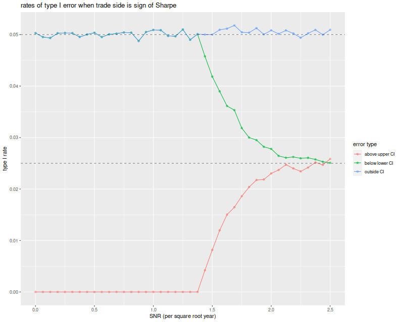
Although the type I error rate is maintained, the 'violations' of the confidence interval can be asymmetric. When the Signal Noise ratio is large (in absolute value), type I errors tend to occur on both sides of the confidence interval equally, because the Sharpe is usually the same sign as the Signal-Noise ratio. When the Signal-Noise ratio is near zero, however, typically the type I errors occur only on the lower side. (This must be the case when the Signal-Noise ratio is exactly zero.) Of course, since the Signal-Noise ratio is the unknown population parameter, you do not know which situation you are in, although you have some hints from the observed Sharpe ratio.
Before moving on, here we test the symmetric confidence intervals. We vary the Signal Noise ratio from 0 to 2.5 in 'annual units', draw two years of daily normal returns with that Signal-Noise ratio, pick a side of the trade based on the sign of the Sharpe ratio, then build symmetric confidence intervals using the standard error estimator $\sqrt{(1 + \hat{\zeta}^2/2)/n}$. We build the 95% confidence intervals, then note any breaches of the upper and lower confidence bounds. We repeat this 10000 times for each choice of SNR.
We then plot the type I rate for the lower bound of the CI, the upper bound and the total type I rate, versus the Signal Noise ratio. We see that the total empirical type I rate is very near the nominal rate of 5%, and this is entirely attributable to violations of the lower bound up until a Signal Noise ratio of around 1.4 per square root year. At around 2.5 per square root year, the type I errors are observed in equal proportion on both sides of the CI.
suppressMessages({
  library(dplyr)
  library(tidyr)
  library(future.apply)
})
# run one simulation of normal returns and CI violations
onesim <- function(n,pzeta,zalpha=qnorm(0.025)) {
    x <- rnorm(n,mean=pzeta,sd=1)
    sr <- mean(x) / sd(x)
    se <- sqrt((1+0.5*sr^2)/n)
    cis <- abs(sr) + se * abs(zalpha) * c(-1,1)
    pquant <- sign(sr) * pzeta
    violations <- c(pquant < cis[1],pquant > cis[2])
}
# do a bunch of sims, then sum the violations of low and high;
repsim <- function(nrep,n,pzeta,zalpha) {
  jumble <- replicate(nrep,onesim(n=n,pzeta=pzeta,zalpha=zalpha))
  retv <- t(jumble)
  colnames(retv) <- c('nlo','nhi')
  retv <- as.data.frame(retv) %>%
        summarize_all(.funs=sum)
    retv$nrep <- nrep
    invisible(retv)
}
manysim <- function(nrep,n,pzeta,zalpha,nnodes=7) {
  if (nrep > 2*nnodes) {
        plan(multisession, workers = 7)
    # do in parallel.
    nper <- table(1 + ((0:(nrep-1) %% nnodes)))
    retv <- future_lapply(nper,function(aper) repsim(nrep=aper,n=n,pzeta=pzeta,zalpha=zalpha)) %>%
      bind_rows() %>%
            summarize_all(.funs=sum)
        plan(sequential)
  } else {
    retv <- repsim(nrep=nrep,n=n,pzeta=pzeta,zalpha=zalpha)
  }
    # turn sums into means
    retv %>%
        mutate(vlo=nlo/nrep,vhi=nhi/nrep) %>%
        dplyr::select(vlo,vhi)
}

# run a bunch
ope <- 252
nyr <- 2
alpha <- 0.05

# simulation params
params <- data_frame(zetayr=seq(0,2.5,by=0.0625)) %>%
    mutate(pzeta=zetayr/sqrt(ope)) %>%
    mutate(n=round(ope*nyr))

# run a bunch
nrep <- 100000
set.seed(4321)
system.time({
results <- params %>%
  group_by(zetayr,pzeta,n) %>%
    summarize(sims=list(manysim(nrep=nrep,nnodes=7,
                                pzeta=pzeta,n=n,zalpha=qnorm(alpha/2)))) %>%
  ungroup() %>%
  tidyr::unnest()
})
suppressMessages({
  library(dplyr)
  library(tidyr)
  library(ggplot2)
})
ph <- results %>%
    mutate(vtot=vlo+vhi) %>%
    gather(key=series,value=violations,vlo,vhi,vtot) %>%
    mutate(series=case_when(.$series=='vlo' ~ 'below lower CI',
                                                    .$series=='vhi' ~ 'above upper CI',
                                                    .$series=='vtot' ~ 'outside CI',
                                                    TRUE ~ 'error')) %>%
    ggplot(aes(zetayr, violations, colour=series)) +
    geom_line() + geom_point(alpha=0.5) +
    geom_hline(yintercept=c(alpha/2,alpha),linetype=2,alpha=0.5) +
    labs(x='SNR (per square root year)',y='type I rate',
             color='error type',title='Rates of type I error when trade side is sign of Sharpe')
print(ph)
A Bayesian Donut?
Of course, this strategy seems a bit unrealistic: what's the point of constructing confidence intervals if you are going to trade the asset no matter what the evidence? Instead, consider a fund manager whose trading strategies are all above average: she/he observes the Sharpe ratio of a backtest, then only trades a strategy if $|\hat{\zeta}| \ge c$ for some sufficiently large $c$, and picks a side based on $\operatorname{sign}\left(\hat{\zeta}\right)$. This is a 'donut'.
Conditional on observing $|\hat{\zeta}| \ge c$, can one construct a reliable confidence interval on $\operatorname{sign}\left(\hat{\zeta}\right) \zeta$? Perhaps our fund manager thinks there is no point in doing so if $c$ is sufficiently large. I think to do so you have to make some assumptions about the distribution of $\zeta$ and rely on Baye's law. We did not say what would happen if the junior quant at this shop developed a strategy where $|\hat{\zeta}| < c$, but presumably the junior quants were told to keep working until they beat the magic threshold. If the junior quants only produce strategies with small $\zeta$, one suspects that the $c$ threshold does very little to reject bad strategies, rather it just slows down their deployment. (In response the quants will surely beef up their backtesting infrastructure, or invent automatic strategy generation.)
Generalizing to higher dimensions
The real interesting question is what this looks like in higher dimensions. Now one observes $p$ assets, and is to construct a portfolio on those assets. Can we construct good confidence intervals on the Sharpe ratio of the chosen portfolio? In this setting we have many more possible choices, so a general purpose analysis seems unlikely. However, if we restrict ourselves to the Markowitz portfolio, I suspect some progress can be made. (Although I have been very slow to make it!) I hope to purse this in a followup blog post.
Click to read and post comments