In a previous blog post I considered the "deflated Sharpe ratio" of Bailey and López de Prado
and found it quite lacking: it comes with zero theoretical justification and fails to do anything sensible in practice.
Here I consider a simple conditional estimator for the problem targeted by the deflated Sharpe ratio, one which actually
exhibits good coverage.
We start from the same setup as the deflated Sharpe ratio:
historical performance of a large number of strategies.
The historical performance is the sum of skill and luck, both of which are
normally distributed. (The normality of luck is a simplification we ignore for this blog post.)
One selects the strategy with the best in-sample performance, then performs
inference on the skill of that strategy.
In this case the skill is population Sharpe ratio, while the in-sample performance is the sample Sharpe ratio.
Again, you want a strategy with high skill, but can only select on skill plus luck.
In our case the luck is the noise of the in-sample Sharpe ratio around the
signal-noise ratio.
The magnitude of this noise is controlled mostly by the length of the backtest period,
and is approximately $1/T$ where $T$ days of backtested returns are observed.
So we suppose that the skill of the $i$th strategy, $\mu_i$ is normally distributed:
$$
\mu_i \sim \mathcal{N}\left(\mu, \sigma^2_s\right).
$$
We then observe the in-sample performance $x_i$ which is the sum of $\mu_i$ and a normal error:
$$
\left(x_i - \mu_i\right) \sim \mathcal{N}\left(0, \sigma^2_l\right).
$$
We assume that the $\left\{x_i, x_i-\mu_i\right\}$ are all independent of each other.
We write the vector of the $x_i, \mu_i$ as a bivariate normal:
$$
\left[\begin{array}{c} \mu_i\\ x_i\end{array}\right] \sim \mathcal{N}\left(\left[\begin{array}{c}\mu\\ \mu\end{array}\right], \left[\begin{array}{cc} \sigma_s^2 & \sigma_s^2 \\ \sigma_s^2 & \sigma_l^2 + \sigma_s^2\end{array}\right] \right)
$$
Let $\gamma = \sigma_l^2 / \left(\sigma_l^2 + \sigma_s^2\right)$ be the amount of total variation ascribed to luck.
Then conditional on observing $x_i = v$ for some value $v$ we have that $\mu_i$ is conditionally normal with distribution:
$$
\mu_i\left|x_i = v \right. \sim \mathcal{N}\left(\gamma\mu + \left(1 - \gamma\right)v, \gamma \sigma^2_s\right).
$$
This is a good start, but it would seem that to estimate $\mu_i$ from this we would need to know $\mu$.
We could assume this as part of a null, but then our test would test both that null value and the value of $\mu_i$, when
we are only really concerned with the value of $\mu_i$.
Instead, we would like to estimate $\mu$ via plugging in the sample mean $\bar{x}$.
This slightly complicates matters, depending on how you perform the correction.
I have found that everything works out nicely if you subtract the sample mean all around.
Letting $\bar{x} = n^{-1} \sum_j x_j$, we note that $\bar{x}$ is correlated with $x_i$,
it is simple to show that
$$
\left[\begin{array}{c} \mu_i - \bar{x}\\ x_i - \bar{x}\end{array}\right] \sim \mathcal{N}\left(\left[\begin{array}{c}0\\ 0\end{array}\right], \left[\begin{array}{cc} \frac{n-1}{n}\sigma_s^2 + \frac{1}{n}\sigma_l^2 & \frac{n-1}{n}\sigma_s^2 \\ \frac{n-1}{n}\sigma_s^2 & \frac{n-1}{n}(\sigma_l^2 + \sigma_s^2)\end{array}\right] \right).
$$
Now if we condition on the observed value of $x_i - \bar{x}$ taking some value $v$ we have
$$
\mu_i - \bar{x} \left| x_i - \bar{x} = v \right. \sim \mathcal{N}\left((1-\gamma)v, \frac{n-1}{n}\gamma\sigma_s^2 + \frac{1}{n}\sigma_l^2 \right).
$$
Thus a conditional $\alpha$-confidence bound on $\mu_i$ conditional on observing $x_i, \bar{x}$ is
$$
\bar{x} + (1-\gamma)(x_i - \bar{x}) + z_{\alpha} \sqrt{\frac{n-1}{n}\gamma\sigma_s^2 + \frac{1}{n}\sigma_l^2},
$$
where $z_{\alpha}$ is the $\alpha$ quantile of the standard normal.
This is all just basic probability and being careful with algebra.
But note that when we conditioned on $x_i$ taking a certain value,
we said nothing about the selection procedure.
In the problem we are targeting, $i$ was selected because it is the argmax of the $x$, which is to say
$x_i \ge x_j$ for all $j$.
(Equivalently $x_i - \bar{x} \ge x_j - \bar{x}$ for all $j$, which is the actual selection we performed.)
It turns out that the ordering is irrelevant because we are conditioning on the value of $x_i$ anyway.
This is apparently implied by a theorem of Kaufmann and Reiss, but I do not understand the proof yet.
Let's confirm this empirically. We simulate the $\mu_i, x_i$ values, find the argmax of the $x_i$,
and look at the associated $\mu_i$. Because this is a simulation we have access to the $\mu_i$.
We compute what should be a standard normal
$$
z = \frac{\mu_i - \left(\bar{x} + (1-\gamma)(x_i - \bar{x})\right)}{\sqrt{\frac{n-1}{n}\gamma\sigma_s^2 + \frac{1}{n}\sigma_l^2}},
$$
then compute the normal CDF of that thing.
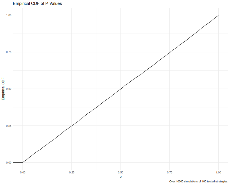
We plot the empirical CDF of the putative p-values.
If our theory is correct this should look like the line segment from $(0,0)$ to $(1,1)$.
In the plot below we see that indeed this is the case.
I have tweaked the $n, \sigma_l^2, \sigma_s^2$ a few times and found that uniformity is not affected by these.
simit <- function(n, ss2, sl2=1.0, mu=5.0) {
    gamma <- sl2 / (sl2 + ss2)
    mu <- rnorm(n, mean=mu, sd=sqrt(ss2))
    x <- rnorm(n, mean=mu, sd=sqrt(sl2))
    xbar <- mean(x)
    iidx <- which.max(x)
    mui <- mu[iidx]
    xi <- x[iidx]
    nmu <- xi - gamma * (xi - xbar)
    nv2 <- (ss2*(n-1)*gamma/n) + (sl2/n)
    zval <- (mui - nmu) / sqrt(nv2)
    pval <- pnorm(zval)
    return(c(mui=mui, xi=xi, xbar=xbar, zval=zval, pval=pval))
}
nstrat <- 100
nsim <- 1e4
set.seed(1234)
blah <- replicate(nsim,simit(nstrat, ss2=0.3, sl2=0.2)) %>% t() %>% tibble::as_tibble()
library(ggplot2)
ph <- blah %>%
    ggplot(aes(x=pval)) +
    stat_ecdf() +
    labs(title='Empirical CDF of P Values',x='p',y='Empirical CDF',
         caption=paste0('Over ',nsim,' simulations of ',nstrat,' tested strategies.'))
print(ph)
I was initially surprised that this worked, because it seems like it would
not deal properly with the selection pressure.
On reflection,
I think it is helpful to consider the two extremes of $\gamma$.
When $\gamma=0$ we basically have spread in skill with no noise from luck.
In that case we should observe that $\mu_i=x_i$.
Our confidence bound becomes
$$
\bar{x} + (x_i - \bar{x}) + z_{\alpha} \sqrt{\frac{1}{n}\sigma_l^2},
$$
but since $\sigma_l=0$ when $\gamma=0$, this is indeed just $x_i$.
When $\gamma=1$ we have essentially no spread in skill and the noise of
luck dominates. In this case all the $\mu_i$ are the same and equal to $\mu$,
so we are better off estimating $\mu_i$ with $\bar{x}$, which has lower
variance than $x_i$ alone (though technically $x_i$ contributes to $\bar{x}$).
Our confidence bound becomes
$$
\bar{x} + z_{\alpha} \sqrt{\frac{1}{n}\sigma_l^2},
$$
which just reflects the standard error around the sample mean, exactly as I would expect.
Compared to the DSR
In our previous blog post we performed a number of simulations on the DSR:
spawn a population of true Sharpe ratios, simulate observed Sharpe ratios, select the strategy
based on the in-sample Sharpe, compute the DSR, return the true Sharpe of the selected strategy
and the DSR. Upon performing this simulation thousands of times we get some empirical estimate
of how well the DSR performed.
Here we will repeat those experiments, but consider our conditional estimator as well.
We simulate using some the values of some parameters from the original DSR paper.
As in the original DSR paper,
we assume 250 trading days per year,
let $\sigma_s^2 + \sigma_l^2 = 0.5$ in "annualized units", let $T = 1250$ days (5 years at this cadence),
assume returns are normally distributed, and fix $n = 100$.
In addition to the DSR, we perform our conditional estimation, tuning it to conditionally test
whether the true Sharpe is negative.
To match the directional sense of the DSR we look at the upper tail CDF so that larger values mean
the strategy is likely better; we will (conditionally) reject the hypothesis that the strategy is
bad when our statistic is large, larger than $1 - \alpha$ for some threshold $\alpha$.
First the simulations.
One oddity of note is that we set $\mu$ to be somewhat negative:
If we set it to zero, there are few observed cases where the selected strategy is actually bad,
and we have to infer the performance of these statistics based on a very small basis.
Even with the value we set here, we actually selected a bad strategy in only approximately a quarter
of the simulations.
exp_max_sr <- function(N) {
    mascher <- 0.5772156649
    (1 - mascher) * qnorm((1/N), lower.tail=FALSE) + mascher * qnorm(exp(-1)/N, lower.tail=FALSE)
}
dsr <- function(sr, T, N, Vsrs, Esrs=0, gamma3=0, gamma4=3, ...) {
    sr0 <- Esrs + sqrt(Vsrs) * exp_max_sr(N)
    serr <- sqrt((1 - gamma3 * sr + (gamma4 - 1)/4*sr**2) / (T-1))
    pnorm((sr - sr0) / serr, ...)
}
condest <- function(sr, srbar, n, ss2, sl2, test_snr=0, ...) {
  gamma <- sl2 / (sl2 + ss2)
  nmu <- sr - gamma * (sr - srbar)
  nv2 <- (ss2*(n-1)*gamma/n) + (sl2/n)
  return(pnorm(test_snr, mean=nmu, sd=sqrt(nv2), ...))
}
#' perform a number of simulations of normal skill plus normal luck,
#' compute the DSR on the results, return the SNR of the strategy
#' selected for having maximal sharpe, along with that maximal sharpe and the DSR statistic.
#' also compute the conditional threshold.
sim_machine <- function(T, n, sigmasq_tot, mu=0, nsims=100000, dpy=250) {
  require(tibble,quietly=TRUE)
  sigma_luck_day <- sqrt(1/T)
  sigma_tot_day <- sqrt(sigmasq_tot / dpy)
  sigma_skill_day <- sqrt(sigma_tot_day^2 - sigma_luck_day^2)

  simvals <- replicate(nsims, {
    skills <- rnorm(n, mean=mu, sd=sigma_skill_day)
    srs <- rnorm(length(skills), mean=skills, sd=sigma_luck_day)
    maxsr <- max(srs)
    nidx <- which.max(srs)
    selskill <- skills[nidx]
    dsrv <- dsr(maxsr, T, N=n, Vsrs=sigma_tot_day^2)
    srbar <- mean(srs)
    condp <- condest(maxsr, srbar, n=n, ss2=sigma_skill_day^2, sl2=sigma_luck_day^2, test_snr=0, lower.tail=FALSE)
    c(skill=selskill, dsr=dsrv, maxsr=maxsr, condp=condp)
  })
  tibble::as_tibble(t(simvals))
}

T <- 1250
n <- 100
sigmasq_tot <- 0.5
set.seed(1234)
results <- sim_machine(T=T, n=n, sigmasq_tot=sigmasq_tot, mu=-0.05, nsims=5e6)
Now we analyze the results.
Because our conditional procedure is, well, conditional, we will not look at these from the usual frequentist lens of type I and type II error rates.
Instead we will condition on the statistic taking a certain value, then compute the proportion of the time
the selected strategy is bad (i.e. has a negative population Sharpe ratio).
We expect that when our statistic is large, the number of such "False Discoveries" should be low.
In fact we would like that the false discovery rate is one minus our conditional statistic. (Recall we flipped the sign so more is better, to match DSR.)
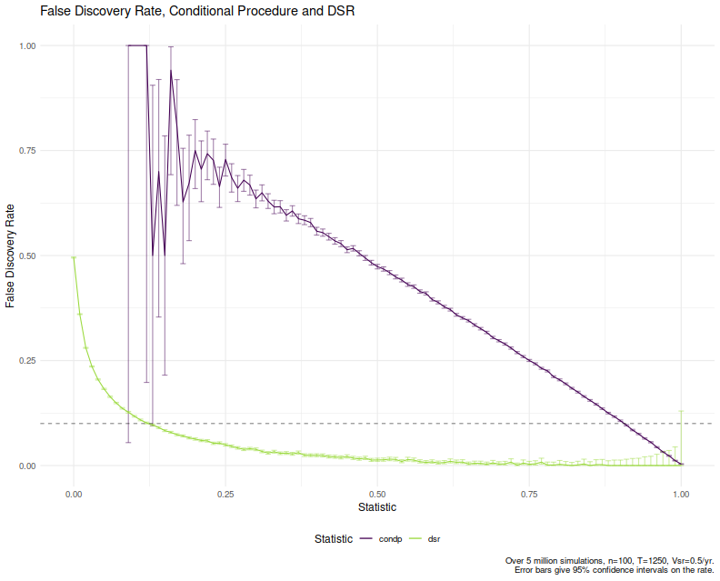
Here is that plot for the 5 million simulations.
We plot a horizontal line at 0.10.
From this plot it would seem that to achieve a 10% FDR using the DSR
we would have to accept a strategy (reject the null) whenever DSR is bigger than around 0.125.
For the conditional procedure the value appears to be just around 0.90, as we would expect.
From this plot we see that the conditional procedure approximately controls the False Discovery Rate,
at least for small FDR rates.
That is, if you wanted to ensure your FDR was below 5 percent, say, you would require the conditional
procedure to produce a value of 0.95 before trading.
It is not clear to me why the line here deviates from the $y=1-x$ line at all.
In contrast to the simulations above, I suspect that the issue is that the "p value" of the
conditional procedure is not independent of the statistic's value, and that causes the procedure
to be somewhat conservative.
Compared to the DSR, however, this is a second order problem.
compute_rejrates <- function(stacked_results, conf.level=0.95, dsr_thresh=0.95) {
  stacked_results %>%
    group_by(stat_group, stat) %>%
      summarize(`Bad Strategy`=sum(skill < 0), Total=n()) %>%
    ungroup() %>%
    mutate(`False Discovery`=`Bad Strategy` / Total) %>%
    mutate(conf.lo=mapply(function(x, n)  {prop.test(x, n, conf.level=conf.level)$conf.int[1]}, `Bad Strategy`, Total)) %>%
    mutate(conf.hi=mapply(function(x, n)  {prop.test(x, n, conf.level=conf.level)$conf.int[2]}, `Bad Strategy`, Total))
}
bind_rows(condp=results %>%
    mutate(stat_group=round(condp, 2)),
  dsr=results %>%
    mutate(stat_group=round(dsr, 2)),.id='stat') %>%
  compute_rejrates() %>%
  ggplot(aes(stat_group,`False Discovery`,group=stat,color=stat)) +
  geom_errorbar(aes(ymin=conf.lo,ymax=conf.hi),alpha=0.5) +
  geom_line() +
  geom_hline(yintercept=0.10,linetype='dashed',alpha=0.5) +
  labs(x='Statistic',y='False Discovery Rate',
       title='False Discovery Rate, Conditional Procedure and DSR',
       color='Statistic',
       caption='Over 5 million simulations, n=100, T=1250, Vsr=0.5/yr.\nError bars give 95% confidence intervals on the rate.')
Summary
We crafted a conditional test statistic that, conditional on observing the maximum and mean of the in-sample Sharpe ratios,
is approximately uniformly distributed when the true Sharpe of the selected strategy is zero.
In contrast to the DSR, which is wildly miscalibrated, it approximately controls for the False Discovery Rate:
if you wish to have a False Discovery Rate less than $\beta$, you should only trade a strategy when this statistic is greater than $1-\beta$.
Our statistic only requires the max and mean Sharpe, the number of strategies and the variance of the skill and the luck.
I believe the procedure can be adapted to the case of general correlation structure on the noise.
This could have been a blog post
An interesting fact about our conditional procedure is that it does not rely at all on the asymptotic maximum of the normal distribution,
the so-called "False Strategy Theorem" that López de Prado has been flogging in four-plus papers.
Instead it seems to smooth between the two extremes of all-luck and all-skill cases,
matching our intuition for both of those, using the sample mean and maximum.
The reason this is just a blog post and not four papers is not just because the derivation took me less than an hour,
but mostly because I don't think the problem setup is a good match for reality.
As I complained in the previous blog post, the assumption that skill is normally distributed is a poor match
for reality in my view.
Moreover, I would expect that strategies are parametrized by some knobs which control both their population Sharpe
and how correlated their backtests are, while the setup to this problem ignores that altogether.
References
- Bailey, David H. and López de Prado, Marcos. 2014. The Deflated Sharpe Ratio: Correcting for Selection Bias, Backtest Overfitting and Non-Normality
Journal of Portfolio Management, 40(5): 94-107. (40th Anniversary Special Issue), DOI: 10.2139/ssrn.2460551
- Arnold, B. C., Balakrishnan, N. and Nagaraja, H. N. 2008. A First Course in Order Statistics, SIAM.
- Kaufmann, E. and Reiss, R.-D. 1992. On conditional distributions of nearest neighbors
Journal of Multivariate Analysis, 42(1): 67-76.
Click to read and post comments
It is commonplace to observe that developing profitable investment strategies is difficult.
Quant strategists are often driven to search over a large number of potential strategies,
backtesting hundreds or thousands before selecting a potential candidate for trading.
Given the relatively short history of available relevant data, quants often have to reason about
their selected strategy using the same data used to select the strategy, a sure recipe for all
kinds of biases and suboptimal decisions.
I have studied this problem quite a bit, and written about it elsewhere.
In my research I have come across the "Deflated Sharpe Ratio" more than once, but had never taken it seriously.
From reading the abstract of the original paper
I thought it was just some kind of heuristic, instead of a statistical procedure.
However, it has blossomed out into a small constellation of papers, with the intersected authorship consisting solely
of Marcos López de Prado, Risk.net's 2021 Buy-Side Quant of the Year.
As of writing this blog post the original paper has over 270 citations on google scholar,
not all of them self-citations, with over 90 in the first half of 2026 alone,
and a more extensive Wikipedia entry
than the Sharpe ratio.
The deflated Sharpe ratio has lodged itself in the firmament of quantitative finance, but how does it work and what does it do?
At a high level, the deflated Sharpe ratio procedure imagines that one observes
historical performance of a large number of strategies.
We can decompose historical performance as a sum of skill and luck.
One then selects the strategy with the best in-sample performance, then performs
some kind of inference on the skill of that strategy.
In this case the skill can be quantified by the population Sharpe ratio
(what I call the "signal-noise ratio").
One wants a strategy with high skill, since you cannot control luck:
high skill leads to the best expected performance out-of-sample.
In our case the luck is the noise of the in-sample Sharpe ratio around the
signal-noise ratio.
The magnitude of this noise is controlled mostly by the length of the backtest period,
and is approximately $1/T$ where $T$ days of backtested returns are observed.
The setup to the original DSR paper imagines that the distribution of sample
Sharpe ratios is Gaussian with mean zero and variance $\sigma_s^2 +
\sigma_l^2$,
where $\sigma_s^2$ is the variance of the skill part, and $\sigma_l^2$ is the
variance of the luck part, equal to around $1/T$.
This is a simplified representation of the DSR procedure, ignoring some
corrections for skew and kurtosis of returns, which will have no bearing on our
analysis.
The DSR procedure is built on the "False Strategy Theorem" which gives
a formula for the asymptotic expected value of the maximum of $n$ i.i.d.
standard Gaussian random variables. We can think of this as just a function of
$n$, call it $f(n)$.
Now let $\hat{\zeta}_i$ be the observed Sharpe ratios of the $i$th backtest,
and suppose we reorder them so that $\hat{\zeta}_n$ is the largest in-sample value.
We are trying to perform inference on the skill of this strategy.
The DSR is basically computed as
$$
DSR = \Phi\left(\frac{\hat{\zeta}_n - \sqrt{\sigma_s^2 + \sigma_l^2}f(n)}{\sigma_l}\right).
$$
That is, we subtract the (approximate) expected value of the maximum of skill
plus luck,
divide by the spread of the luck, then feed the result through the CDF of the
normal distribution.
In the original 2014 paper, the authors allude to the DSR being used as a
statistical procedure.
They give a number of example computations, and talk about rejecting a null
hypothesis based on whether the computed DSR exceeds 0.95 or not.
(A larger value of the DSR apparent casts doubt on the null hypothesis.)
The 2018 paper by López de Prado and Lewis defines the DSR as
"the probability that the true SR exceeds a user-defined benchmark level
$SR^*$, where that level is
adjusted to reflect the multiplicity of trials."
Ignoring that frequentists do not assign probabilities to underlying parameters,
the intention is fairly clear that DSR is to be interpreted as a p-value.
Wait, What?
I had a number of concerns after reading this paper.
Among them:
-
The assumption that sample Sharpe ratios are normally distributed seems
indefensible in practice, and is likely load-bearing.
There are two issues here.
Even if one assumes that returns are well behaved
(independent Gaussian, say), the Sharpe ratio is fat-tailed.
The distributional shape of skill will not change this.
Because the "False Strategy Theorem" is based on asymptotics of the normal
distribution, and because we are looking at extremal values, the
fat-tailedness of the sample Sharpes is likely to break the expected value
used in the DSR computation. The expectation subtracted in the numerator of DSR is probably wrong.
The other issue with this assumption is that skill is unlikely to be
normally distributed, which is pretty much required if skill plus luck is
normally distributed. Quants tend to test small variations on a number of
different heterogenous strategies. Normality seems like a very poor model for
how skill is distributed.
The authors of the original paper ignore this issue, but it seems like it is addressed
in the followup paper
by López de Prado and Lewis.
Needless to say the followup paper requires some results from the original
paper that are demonstrably wrong.
-
The definition of the DSR is quite odd.
The numerator $\hat{\zeta}_n - \sqrt{\sigma_s^2 + \sigma_l^2}f(n)$
should be approximately zero mean if the expected value of the sample Sharpe ratios is zero,
but larger otherwise.
How much larger is hard to say, but it does not seem that it should depend
only on $\sigma_l$, which is what we divide it by.
In fact, it seems that the intent is to measure how many "luck units"
away we are from what we suspect should be zero.
The problem is that the maximal sample Sharpe $\hat{\zeta}_n$ has both skill
and luck in it, and we cannot just pretend that we maximized over skill and
then had luck-sized noise on top of that.
-
This also raises the issue of what null exactly is putatively being tested
here.
The authors do not state this clearly, in either the original 2014 paper or the
2018 followup.
There are a few obvious choices: the unconditional null, which is that the
expected value of all the sample Sharpe ratios is zero; and the
conditional null which is that the skill of the selected strategy is zero,
symbolically $\zeta_n = 0$, where $n$ is the index of the strategy with the
largest observed sample Sharpe ratio. (We do not know, or exactly care, if
$\zeta_n$ is the largest of the skill values.)
Lastly there is a conditional familywise null which is that the skill of all strategies
is zero (or non-positive), symbolically $\zeta_i = 0$ for all $i$.
We suspect the authors intended to test the conditional null, as the other two
nulls can be tested with standard MHT corrections like Bonferroni.
The two other nulls also do not seem super useful, since they are not strictly about
the skill of the selected strategy.
-
You might be wondering how the authors proved that the DSR is uniform
under the null hypothesis if they did not state the null hypothesis.
I regret to inform there is no proof of this statement.
Instead, the efficacy of DSR for controlling type I errors
rests on the reputation of the authors and the editors of the Journal of
Portfolio Management.
Disproving Uniformity of the DSR
The fact that I could not immediately grasp the justification for the DSR is not real cause for concern.
After all, there are many, many things I do not understand.
However the absence of a proof, or even a hand-wave justification, is troubling from my point of view.
The authors and editors did not seem to think a proof was necessary.
I now believe that no proof was offered because there is no proof, as the statement is clearly false.
Consider the simplified case where there is no spread in skill, $\sigma_s=0$.
In this case all strategies have the same skill
which we assume to be zero.
(Note that if this were true there would be no reason to select among the strategies, but this is the limiting case where spread of luck is much larger than spread of skill.)
The three nulls happen to coincide here, so it does not matter which one the original authors intended.
Suppose that $\sigma_l=1$ by choice of units, so that DSR is defined as
$\Phi\left(\hat{\zeta}_n - f(n)\right)$.
For large $n$ the maximum of $n$ i.i.d. Gaussians tends to a Gumbel distribution.
This is simply not normally distributed, and the DSR should not be uniform under the null.
We can simulate this very easily. We simulate $n$ independent Gaussians, select the maximal one,
subtract the magical value, take the CDF, and get something that should be uniform if we believe the DSR is a p-value.
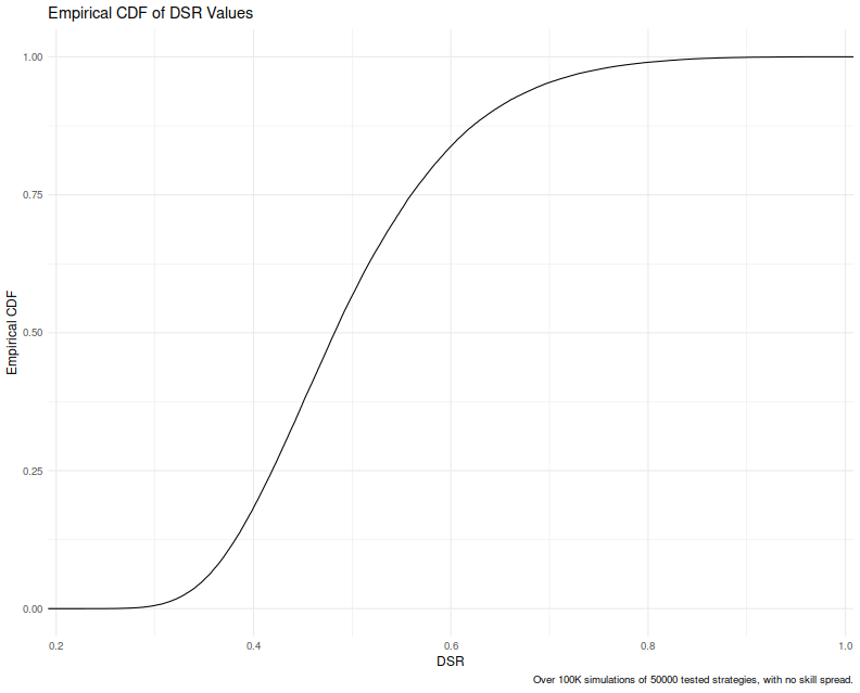
We run this simulation $10^5$ times and
plot the empirical CDF of these putative p-values.
If the DSR were uniform this would be a straight line segment from $(0,0)$ to $(1,1)$.
It clearly is not.
Note that we are simulating $n=50000$ strategies here, so the problem is not the asymptotics:
these are the asymptotics.
In fact, using larger $n$ does not improve the situation.
This is evident from other testing we have done
and is obvious from the asymptotics, since the variance of the maximum of $n$ Gaussians is shrinking in $n$.
This even figures into the 2014 paper of this constellation,
but apparently did not occur to authors of the DSR paper.
exp_max_sr <- function(N) {
    mascher <- 0.5772156649
    (1 - mascher) * qnorm((1/N), lower.tail=FALSE) + mascher * qnorm(exp(-1)/N, lower.tail=FALSE)
}
nstrat <- 50000
limval <- exp_max_sr(nstrat)
set.seed(1234)
simvals <- replicate(1e5,{
  srs <- rnorm(nstrat, mean=0, sd=1)
  dsr <- pnorm(max(srs) - limval)
})
library(tibble)
library(dplyr)
library(ggplot2)
ph <- tibble(sample=simvals) %>%
  ggplot(aes(x=sample)) +
  stat_ecdf() +
  labs(title='Empirical CDF of DSR Values',x='DSR',y='Empirical CDF',caption=paste0('Over 100K simulations of ',nstrat,' tested strategies, with no skill spread.'))
print(ph)
Note that conservatively these simulations require 20 lines of code to execute and plot,
and took 15 minutes to write and execute.
That the original authors never bothered to check this is mind-boggling.
The first DSR paper does contain simulations, but only to check how the mean value of $\hat{\zeta}_n$ compares to the asymptotic value as one varies $n$.
While this is an interesting question, it rather misses the mark.
The problem with DSR, as it turns out, is not that $f(n)$ is inaccurate for small $n$;
rather the issue is that the DSR does not make any sense.
As one can see from the plot above, in some situations we should expect that the probability that DSR exceeds $1-\alpha$ will often be
much smaller than $\alpha$.
To illustrate the issue, we simulate using numbers from the original DSR paper.
As in the original paper,
we assume 250 trading days per year,
let $\sigma_s^2 + \sigma_l^2 = 0.5$ in "annualized units", let $T = 1250$ days (5 years at this cadence),
assume returns are normally distributed, and consider either $n = 88$ or $n = 89$.
First we write a DSR function and confirm that if $\hat{\zeta}_n=2.5$ in annualized units that this DSR function
spits out 0.9505 when $n = 88$, as in the original paper.
exp_max_sr <- function(N) {
    mascher <- 0.5772156649
    (1 - mascher) * qnorm((1/N), lower.tail=FALSE) + mascher * qnorm(exp(-1)/N, lower.tail=FALSE)
}
dsr <- function(sr, T, N, Vsrs, Esrs=0, gamma3=0, gamma4=3, ...) {
    sr0 <- Esrs + sqrt(Vsrs) * exp_max_sr(N)
    serr <- sqrt((1 - gamma3 * sr + (gamma4 - 1)/4*sr**2) / (T-1))
    pnorm((sr - sr0) / serr, ...)
}

dpy <- 250
zeta_n <- 2.5
T <- 1250
n <- 88
sigmasq_tot <- 0.5
# compute and print
print(dsr(zeta_n / sqrt(dpy), T=T, N=n, Vsrs=sigmasq_tot / dpy))
print(dsr(zeta_n / sqrt(dpy), T=T, N=n+1, Vsrs=sigmasq_tot / dpy))
I indeed get 0.9505, as in the original paper.
Moreover, when $n=89$, the DSR falls slightly under 0.95 and,
if we are to believe the narrative of the original paper,
a conscientious investor would fail to reject the null and not invest in the strategy.
Our code matches the code in the paper by visual inspection and spits out the same values,
and we can proceed.
Now we will perform a number of simulations with these values of $T, n$ and noise.
In each of them we will first draw from normally distributed skill,
then add some amount of luck to that.
We will select the "strategy" with the highest combined skill plus luck.
We will compute the DSR on the simulated Sharpe of this strategy.
We then get the actual skill and the DSR value.
This will allow us to test the conditional null by focusing on cases where
the actual skill is either less than zero, or very close to it.
Below we perform the simulations under these values of $T, n, \sigma^2_s$.
#' perform a number of simulations of normal skill plus normal luck,
#' compute the DSR on the results, return the SNR of the strategy
#' selected for having maximal sharpe, along with that maximal sharpe and the DSR statistic.
sim_machine <- function(T, n, sigmasq_tot, nsims=100000, dpy=250) {
  require(tibble,quietly=TRUE)
  sigma_luck_day <- sqrt(1/T)
  sigma_tot_day <- sqrt(sigmasq_tot / dpy)
  sigma_skill_day <- sqrt(sigma_tot_day^2 - sigma_luck_day^2)

  simvals <- replicate(nsims, {
    skills <- rnorm(n, mean=0, sd=sigma_skill_day)
    srs <- rnorm(length(skills), mean=skills, sd=sigma_luck_day)
    maxsr <- max(srs)
    nidx <- order(srs, decreasing=TRUE)[1]
    selskill <- skills[nidx]
    dsrv <- dsr(maxsr, T, N=n, Vsrs=sigma_tot_day^2)
    c(skill=selskill, dsr=dsrv, maxsr=maxsr)
  })
  as_tibble(t(simvals))
}

T <- 1250
n <- 88
sigmasq_tot <- 0.5
set.seed(1234)
results <- sim_machine(T=T, n=n, sigmasq_tot=sigmasq_tot, nsims=1e6)
Now we compute the empirical rejection rates.
To avoid "bottoming out", we pretend we are interested in a type I rate of 0.10, so our decision threshold is to
reject when $DSR > 0.9$.
Here we tabulate the empirical rejection proportion for the entire simulation,
which is under the unconditional null,
as well as for those small number (less than 1%!) of cases where the skill of the selected
strategy is non-positive, which is the conditional null.
We compute 95% confidence intervals on the rejection rate based on our simulations,
and tabulate these below.
We see only one rejection at the nominal 0.10 level under the conditional null,
which we observe over 3000 times in 1 million simulations.
For the conditional null the actual rejection rate is around 100 times smaller than the nominal 0.10 rate promised by the DSR.
Under the unconditional null the empirical rejection rate is more like 4%, not the nominal 10%.
We note, however that under this unconditional null there are many cases where the
skill of the selected strategy is quite large, larger than 1.5 in annualized units.
And yet the rejection rate is still small.
#' estimate the rejection rates along with confidence intervals on same
#' assumes the skill has already been grouped into skill_group variable.
compute_rejrates <- function(results, conf.level=0.95, dsr_thresh=0.95) {
  results %>%
    group_by(skill_group) %>%
      summarize(Rejections=sum(dsr > dsr_thresh), Total=n()) %>%
    ungroup() %>%
    mutate(`Rejection Proportion`=Rejections/Total) %>%
    mutate(conf.lo=mapply(function(x, n)  {prop.test(x, n, conf.level=conf.level)$conf.int[1]}, Rejections, Total)) %>%
    mutate(conf.hi=mapply(function(x, n)  {prop.test(x, n, conf.level=conf.level)$conf.int[2]}, Rejections, Total))
}
library(knitr)
bind_rows(results %>%
  mutate(skill_group="unconditional null"),
results %>%
  dplyr::filter(skill < 0) %>%
  mutate(skill_group="conditional null")) %>%
  compute_rejrates(dsr_thresh=0.9) %>%
  rename(`Group`=skill_group) %>%
  knitr::kable(caption='Empirical rejection rates for simulations using 0.9 DSR threshold.', format='markdown', digits=3)
Table: Empirical rejection rates for simulations using 0.9 DSR threshold.
| Group |
Rejections |
Total |
Rejection Proportion |
conf.lo |
conf.hi |
| conditional null |
1 |
3361 |
0.000 |
0.000 |
0.002 |
| unconditional null |
41627 |
1000000 |
0.042 |
0.041 |
0.042 |
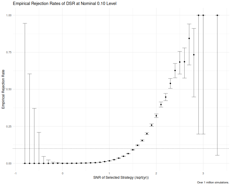
To get a feel for how the DSR rejects at the nominal 0.10 level,
we group cases by their underlying skill, rounding to the nearest 0.1 in annualized units.
We compute the empirical rejection rates of the DSR along with (pointwise, not familywise)
95% confidence intervals, which we plot here.
We see that the empirical rejection rate does not exceed the nominal level
until the skill is around 1.5 in annualized units.
The DSR has apparently very low power when the skill is less than 2 in annualized units.
rejrates <- results %>%
  mutate(skill_group=round(sqrt(250)*skill, 1)) %>%
  compute_rejrates(dsr_thresh=0.90)
ph <- rejrates %>%
  ggplot(aes(skill_group, `Rejection Proportion`, ymin=conf.lo, ymax=conf.hi)) +
  geom_point() +
  geom_hline(yintercept=0.1,linetype="dotted") +
  geom_errorbar(alpha=0.5) +
  labs(x='SNR of Selected Strategy (/sqrt(yr))',
       y='Empirical Rejection Rate',
       title='Empirical Rejection Rates of DSR at Nominal 0.10 Level',
       caption='Over 1 million simulations.')
print(ph)
Steelmanning the DSR
Note that in our simulations we found that the type I rate of DSR seems to be quite smaller than the nominal rate.
Toying with the parameters, we have not found cases where the empirical rejection rate exceeds the nominal rate,
which is to say we suspect that the DSR is uniformly conservative.
It is not uncommon in statistical practice to employ a statistic that depends on some unobserved nuisance parameter.
In that case one usually identifies a least favorable configuration, which is some value of the unobserved nuisance parameter
at which the type I rate is maximized under the null, then calibrate the procedure to that case.
The guarantees of the procedure then become an upper bound on the type I rate.
Could this rescue the DSR?
First note that the original authors do not make this claim.
López de Prado and Lewis do not make that claim either, instead they use DSR as if it were uniform under the null.
Second, it is easy to establish that the distribution of the DSR under the null depends not on an unobserved nuisance parameter,
but on the observed value of $n$.
The DSR simply has more spread for smaller $n$.
This means that for a fixed value of the skill of the selected strategy,
the DSR is more likely to reject for small $n$ than for large $n$.
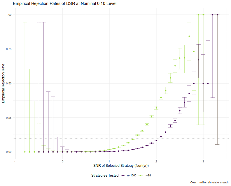
We confirm this experimentally below by repeating the above experiments but setting $n=1000$.
We plot the conditional empirical rejection rates at the nominal 0.10 level for both sets of simulations
and see a much higher rejection rate for the case where $n=88$.
Presumably the "least favorable configuration", then, would be $n=1$, where we do not trust $f(n)$ to be any good.
However, this variable rejection rate is going to be a serious problem if one
attempts to use the DSR result for different normally distributed clusters of skill,
as do López de Prado and Lewis.
Their proposed solution is built on very shaky foundations, and I would not trust it at all:
it will preferentially surface small clusters over large clusters for no good reason.
results2 <- sim_machine(T=T, n=1000, sigmasq_tot=sigmasq_tot, nsims=1e6)
rejrates2 <- results2 %>%
  mutate(skill_group=round(sqrt(250)*skill, 1)) %>%
  compute_rejrates(dsr_thresh=0.90)
ph <- bind_rows(rejrates %>% mutate(n=88),
          rejrates2 %>% mutate(n=1000)) %>%
  mutate(experiment=paste0("n=",n)) %>%
  ggplot(aes(skill_group, `Rejection Proportion`, ymin=conf.lo, ymax=conf.hi,
             color=experiment, group=experiment)) +
  geom_point() +
  geom_hline(yintercept=0.1,linetype="dotted") +
  geom_errorbar(alpha=0.5) +
  labs(x='SNR of Selected Strategy (/sqrt(yr))',
       y='Empirical Rejection Rate',
       title='Empirical Rejection Rates of DSR at Nominal 0.10 Level',
       color='Strategies Tested',
       caption='Over 1 million simulations each.')
print(ph)
In one last-ditch effort to steelman the DSR, perhaps we should just assume that one always
uses it for fixed values of $n$ and $T$, and then performs simulations like the ones I have done here
to get the proper threshold value of DSR to reject at a given type I rate.
There are so many things wrong with this approach, however:
- It requires the user to run a bunch of simulations to fix a broken statistic? Is it not the responsibility of the original authors to do this?
- If you fix the $n$ and $T$, then the DSR is monotonic in $\hat{\zeta}_n$. So if you are going to run these simulations, why waste your time with computing $f(n)$ and the normal CDF? Instead just find threshold values for $\hat{\zeta}_n$ under the conditional null you seek to test, you get the same results. Note that this is just the in-sample Sharpe ratio that these authors have spent five plus papers telling us was biased and useless.
No, there is no rescuing the DSR. Stop using it, it makes no sense, and it does not do what it was advertised to do.
Is DSR a Fraud?
Bailey et al ask a similar question in their paper on "backtest overfitting".
A fraud is an intentional act of deception or a misrepresentation of facts to gain an unfair advantage.
I will stress however, there is no evidence whatsoever of intentional deception here.
The DSR is not a fraud, but it is a misrepresentation of the truth.
In cases like these I employ Hanlon's razor: "Never attribute to malice that which is adequately explained by ignorance".
Writing and publishing the DSR paper(s) without spending even five minutes thinking about whether it is true, or 30 minutes testing it, is in my opinion outright statistical malpractice.
The paper should be retracted, and I will present my case to JPM, though I doubt it will be.
References
- Bailey, David H. and López de Prado, Marcos. 2014. The Deflated Sharpe Ratio: Correcting for Selection Bias, Backtest Overfitting and Non-Normality
Journal of Portfolio Management, 40(5): 94-107. (40th Anniversary Special Issue), DOI: 10.2139/ssrn.2460551
- López de Prado, Marcos and Lewis, Michael J. 2018. Detection of False Investment Strategies Using Unsupervised Learning Methods
Quantitative Finance, 19(9): 1555-1565. DOI: 10.2139/ssrn.3167017 DOI: 10.1080/14697688.2019.1622311
- López de Prado, Marcos and Bailey, David H. 2021. The False Strategy Theorem: A Financial Application of Experimental Mathematics
American Mathematical Monthly, 128(9): 806-817. DOI: 10.1080/00029890.2021.1965068
- Bailey, David H. and Borwein, Jonathan and Borwein, Jonathan and López de Prado, Marcos and Zhu, Qiji Jim. 2014. Pseudo-Mathematics and Financial Charlatanism: The Effects of Backtest Overfitting on Out-of-Sample Performance Notices of the American Mathematical Society, 61(5): 458-471. DOI: 10.2139/ssrn.2308659
Appendix: What Should You Do Instead?
This blogpost is not about me, but I have done research on this problem.
I would be remiss if I did not point readers to my preprint,
which is ostensibly about a procedure which does maintain nominal coverage under the conditional null.
The paper snowballed however and also contains several tests for the unconditional null,
with some analysis of the false discovery rate, etc.
The tests are available in the SharpeR R package as sr_conditional_test and sr_max_test.
By no means do I consider the topic closed, however.
I think the conditional procedure can be improved to have higher power, and am slowly researching and developing a fix.
Click to read and post comments
Some of the research on the problem of "overfitting" of quantitative strategies
(including my own) might be better
described as research on "over-optimism". That is because the analysis
tends to view the strategies as something one stumbles upon, without any
in-sample tinkering. If that is the case, the Sharpe ratio is nearly
unbiased for the signal-noise ratio, and the only statistical sin is
selecting the best strategy among many without some kind of multiple hypothesis
test correction. However, strategies tend to be generated based on some
in-sample overfitting beyond just selection. As an example, suppose you
observed $n$ days of returns on $k$ assets in your universe, then constructed
the Markowitz portfolio based on that data. If your strategy is to hold
that Markowitz portfolio, it is a bit trickier to de-bias the in-sample Sharpe ratio.
For the specific problem of estimating what I call the achieved signal-noise
ratio of the Markowitz portfolio, one can use the Sharpe Ratio Information
Criterion of Paulsen and Söhl.
However, I suspect most practicing quants would fall back to cross validation.
Cross validation is a folk remedy
prescribed to cure all ills, probably beneficial but of unknown efficacy.
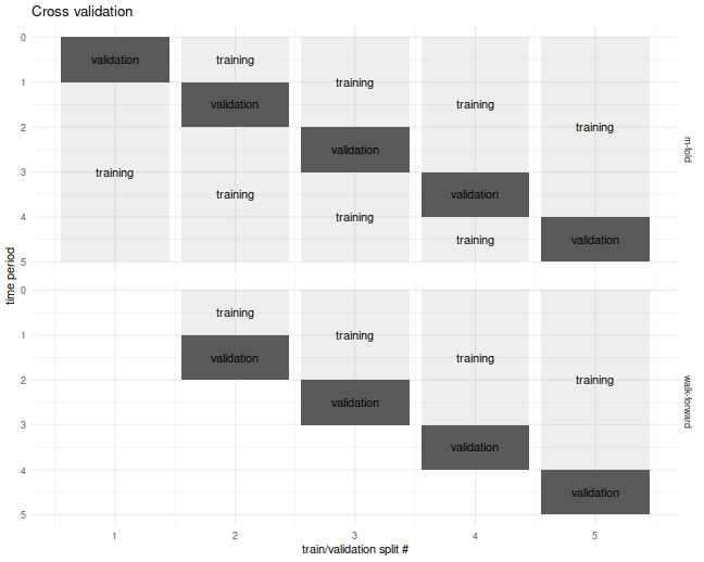
In the usual $m$ fold cross validation, one splits the data into $m$ equally
sized pieces, fits the Markowitz portfolio on all but one of those $m$ pieces,
then simulates returns on that piece. This is repeated holding out each of the $m$
validation sets. The result is a simulated time series over the $n$ days of
data, which one then computes the Sharpe ratio on.
I commonly used a fancier version of cross validation, called walk forward,
where one only estimated the portfolio on data prior to the validation set,
which results in a slightly truncated resultant time series.
The $m$-fold and walk-forward cross validation techniques are illustrated
below for the case of $m=5$ folds.
Cross Validation is Broken?
Although I used cross-validation in this way for years, I never tested it until now.
It seemed "obvious" that it would provide unbiased results.
It turns out I was wrong, as simple simulations will show.
In our set up, cross validation is designed to estimate the achieved
signal-noise ratio. "Achieved" means we are considering the signal-noise ratio
of the sample Markowitz portfolio. This is a quantity that is both random
(depends on the sample) and unobservable (depends on the population mean and
covariance).
In the simulations below I perform $10$-fold regular and walk-forward cross validation,
constructing the Markowitz portfolio on training data, then generating a single
time series of returns, computing the Sharpe on those returns.
I also compute the achieved signal-noise ratio of the Markowitz portfolio
on the whole sample.
I vary the maximal signal-noise ratio of the population, as well as the
number of assets.
For every setting of the population parameters I perform 50000 simulations,
then average the cross validated Sharpes and the achieved signal-noise
ratios over the simulations.
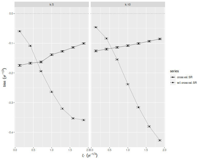
Below I plot the bias of the Sharpes estimated via regular and walk-forward
cross validation, defined as the Sharpe minus the achieved signal-noise ratio.
We see that, in annual terms, both cross validation techniques are severely
biased, and walk-forward gets worse as the maximal signal-noise ratio
increases. The bias is negative, which is to say we _under_estimate the
achieved signal-noise ratio.
suppressMessages({
  library(dplyr)
  library(tidyr)
  library(tibble)
  library(future.apply)
})

# trading days per year
ope <- 252
# compute markowitz portfolio
comp_mp <- function(X) { solve(cov(X),colMeans(X)) }
# compute sr
comp_sr <- function(x,na.rm=TRUE) { mean(x,na.rm=na.rm) / sd(x,na.rm=na.rm) }
# run simulations
simit <- function(n,k,zeta,nsim=1000,nfolds=10) {
  require(future.apply)
  won <- seq(n)
  cvidx <- (won %% nfolds) + 1
  mu <- zeta / sqrt(k)
  vals <- future_replicate(nsim,{
    X <- matrix(rnorm(n*k,mean=mu),ncol=k)
    kfret <- rep(0,n)
    wfret <- rep(NA_real_,n)
    for (folnum in unique(cvidx)) {
      oosi <- cvidx==folnum
      oos <- X[oosi,]
      iis <- X[!oosi,]
      mp <- comp_mp(iis)
      kfret[oosi] <- oos %*% mp
      # walk forward
      iisi <- cvidx < folnum
      if (any(iisi)) {
        iis <- X[iisi,]
        mp <- comp_mp(iis)
        wfret[oosi] <- oos %*% mp
      }
    }
    cv_sr <- comp_sr(kfret)
    wf_sr <- comp_sr(wfret,na.rm=TRUE)
    achieved_snr <- sum(mu * mp) / sqrt(sum(mp^2))
    c(cv_sr,wf_sr,achieved_snr,sqrt(ope)*mean(kfret),sd(kfret))
  })
  setNames(data.frame(sqrt(ope) * t(vals)),c('CV','walkforward','achieved','kf_mean','kf_sd'))
}

nday <- ope*5
nsim <- 50000

params <- crossing(tibble(zeta=seq(0.125,1.875,length.out=7)/sqrt(ope)),tibble(k=c(5,10)))

set.seed(1234)
plan(multicore)
resu <- params %>%
  group_by(zeta,k) %>%
    summarize(foo=list(simit(n=nday,k=k,zeta=zeta,nsim=nsim))) %>%
  ungroup() %>%
  unnest(foo)
plan(sequential)
# aggregate the results:
mresu <- resu %>%
  tidyr::gather(key=series,value=value,-zeta,-k,-achieved) %>%
  mutate(bias=value - achieved) %>%
  group_by(zeta,k,series) %>%
    summarize(emp_bias=mean(bias),
              emp_sbias=sd(bias),
              count=n()) %>%
  ungroup() %>%
  mutate(emp_biase=emp_sbias / sqrt(count))

ph <- mresu %>%
  dplyr::filter(series %in% c('CV','walkforward')) %>%
  mutate(showser=case_when(series=='CV'  ~ 'cross val. SR',
                           series=='walkforward' ~ 'w.f. cross val. SR',
                           TRUE ~ 'error')) %>%
  ggplot(aes(sqrt(ope)*zeta,emp_bias,
             linetype=showser,
             group=interaction(k,showser))) +
  geom_hline(yintercept=0,linetype=3,alpha=0.8) +
  geom_point(aes(shape=showser),alpha=0.9) +
  geom_errorbar(aes(ymin=emp_bias - emp_biase,ymax=emp_bias + emp_biase),width=0.1) +
  geom_line(alpha=0.5) +
  facet_wrap(~k,labeller=label_both) +
  labs(x=expression(zeta['*']~~(yr^{-1/2})),
       y=expression(bias~~(yr^{-1/2})),
       shape='series',
       linetype='series')
print(ph)
Where is the bias?
Despite the relative simplicity of the simulations, I was convinced they
contained a bug. How could cross-validation be so broken?
I tried increasing the number of folds, which only made the problem worse!
In my debugging I noticed that the estimate of the mean return of the
Markowitz portfolio seemed unbiased.
How can one have an unbiased estimate of the mean, but a biased estimate
of the Sharpe ratio?
The answer to that question is that the sample mean and sample standard
deviation are not independent under cross validation.
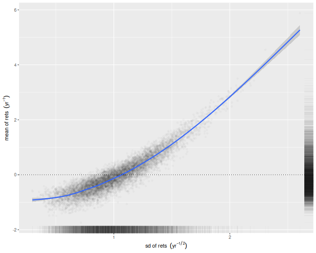
We illustrate that here by performing simulations where the population
mean is the zero vector. For each simulation we compute the numerator and
denominator of the cross-validated Sharpe ratio, namely the mean and
standard deviation of the simulated returns on validation sets.
We then scatter the means versus the standard deviations.
There is a clear correlation here.
I believe this is a well-known effect in cross-validation.
Moreover, if your standard deviation is positively correlated
with your mean, it will clearly bias your Sharpe ratio.
This is simple to understand intuitively, we
leave it as an exercise to show how that bias
is a function of the correlation.
nday <- ope*5
nsim <- 10000

set.seed(1234)
plan(multiprocess)
atz <- simit(n=nday,k=5,zeta=0,nsim=nsim)
plan(sequential)

# scatter em:
ph <- atz %>%
  ggplot(aes(kf_sd,kf_mean)) +
  geom_point(alpha=0.02) +
    stat_smooth() +
    geom_hline(yintercept=0,linetype=3) +
    geom_rug(alpha=0.02,sides='rb') +
  labs(x=expression(sd~of~rets~~(yr^{-1/2})),
       y=expression(mean~of~rets~~(yr^{-1})))
print(ph)
What can be done?
If you intended to trade the Markowitz portfolio, you could probably debias
the cross-validated estimates by some mathematical wizardry.
However, most quants deploy more complicated trading strategies,
which would be harder to analyze.
My only suggestion at the moment is to instead use an average of Sharpes
approach: perform cross-validation as usual, but instead of computing a single
time series of returns, compute the Sharpe ratio on each validation set,
then average them. In a future blog post I will show that this has far less
bias for our toy problem.
Click to read and post comments
Consider the following challenge:
estimate the Signal-Noise ratio of an asset given a single
observation of returns of that asset, $x$.
The task seems impossible: you can easily estimate the mean, but
how are you going to estimate the standard deviation
with just one observation?
Consider, however,
that for most assets the expected value of returns is very small compared to the volatility,
so if you wanted to estimate the variance of returns, $x^2$ would be a good guess.
Thus $\left|x\right|$ would be a passable estimate for the standard deviation.
Given that $x$ is an unbiased estimate of the mean, then
$$
\frac{x}{\left|x\right|} = \operatorname{sign}(x)
$$
is our candidate estimator of the Signal-Noise ratio.
It turns out this will work, up to scaling.
Suppose that returns are Gaussian. Then
$$
E\left[
\operatorname{sign}(x)
\right] = 2\Phi\left(\frac{\mu}{\sigma}\right) - 1
\approx \sqrt{\frac{2}{\pi}} \frac{\mu}{\sigma}.
$$
Thus $\sqrt{\frac{\pi}{2}} \operatorname{sign}(x)$
is a nearly unbiased estimator of the Signal-Noise ratio.
Since this estimator has only two possible values, it is going to be very noisy.
However, if you had $n$ observations $x_t$, you could
average them together as
$$
\check{\zeta} = \frac{1}{n}\sqrt{\frac{\pi}{2}} \sum_{1 \le t \le n}\operatorname{sign}\left(x_t\right).
$$
Call this the sign Sharpe ratio.
Note that it is just a rescaled version of the cringe-worthy "winning days percentage"
statistic some portfolio managers advertise.
There are two obvious problems with the sign Sharpe ratio.
- It is easy to show that the standard error of $\check{\zeta}$ is
$\sqrt{\frac{\pi}{2n}}$, which is about 20% bigger than that
of the moment-based Sharpe ratio.
- It is only nearly unbiased for Gaussian returns, and can have
serious bias for skewed returns.
The latter point is a serious problem. One can easily construct returns
streams with absurdly high or low values of winning days percentage,
and somewhat arbitrary signal-noise ratio.
By using the Edgeworth expansion, one can show that the expected value
of $\check{\zeta}$ is approximately
$$
E\left[
\check{\zeta}
\right] \approx \zeta - \frac{\gamma_1}{6},
$$
where $\zeta=\mu/\sigma$ is the Signal-Noise ratio, and $\gamma_1$ is the
standardized skewness of returns. Of course, if you somehow knew the skew
of returns, you could correct for them.
More interesting would be to find a way to estimate $\gamma_1$ from a
single observation, though I would argue that
$c\operatorname{sign}\left(x\right)$ is probably the best candidate.
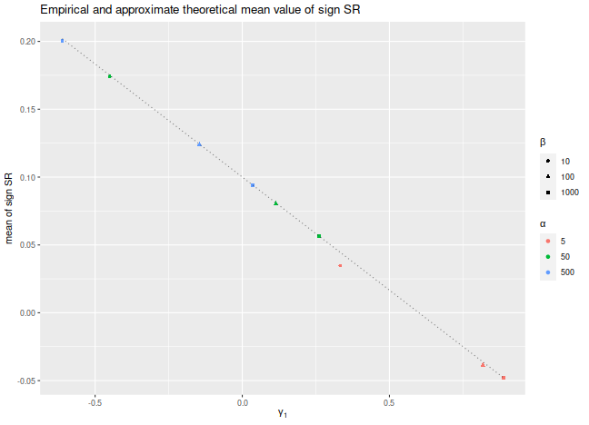
Let's confirm these findings experimentally.
Consider the case where $x_t$ are drawn from a Beta distribution,
shifted to have a fixed mean.
We fix the Signal-Noise ratio to be 0.1, and
tweak the two shape parameters of the Beta distribution,
$\alpha$ and $\beta$, to vary the skewness of returns.
We plot the empirical mean value of $\check{\zeta}$ for
$n=10^7$, along with the approximate theoretical value,
versus the skewness.
We see very good agreement between the two except for the case
where $\alpha$ and $\beta$ are small, where the higher order moments
which we have discarded are no longer negligible.
We would note that this is also likely to be a problem for
real world asset returns.
library(dplyr)
library(tidyr)
library(tibble)
library(ggplot2)

# generate shifted beta variates with a fixed SNR zeta
genb <- function(n,zeta,alpha,beta) {
  mu <- alpha / (alpha+beta)
  sg <- sqrt(alpha*beta/((alpha+beta+1)*(alpha+beta)^2))
  x <- (sg*zeta - mu) + rbeta(n,shape1=alpha,shape2=beta)
}
signsr <- function(x) { sqrt(pi/2) * mean(sign(x)) }

zeta <- 0.1
set.seed(12345)
sims <- crossing(tibble(alpha=c(5,50,500)),tibble(beta=c(10,100,1000))) %>%
  group_by(alpha,beta) %>%
    summarize(simzet=signsr(genb(n=10000000,zeta=zeta,alpha=alpha,beta=beta)),
              skew=2*(beta-alpha)*sqrt(beta+alpha+1)/((alpha+beta+2)*sqrt(alpha*beta))) %>%
  ungroup() %>%
  mutate(esign=zeta - skew / 6)

# plot them:
sims %>%
  ggplot(aes(skew,simzet)) +
  geom_point(aes(color=factor(alpha),shape=factor(beta))) +
  geom_line(aes(y=esign),linetype=3,alpha=0.5) +
  labs(x=expression(gamma[1]),
       y='mean of sign SR',
       title='Empirical and approximate theoretical mean value of sign SR',
       color=expression(alpha),shape=expression(beta))
Is it useful?
The sign Sharpe ratio does not seem useful for estimating the Signal-Noise
ratio: it is too noisy, and is confounded by higher order moments.
However, the challenge of estimating the Sharpe from individual
observations was motivated by difficulties bounding the out-of-sample
Sharpe ratio from the-in-sample Sharpe ratio using something
like VC dimension or Rademacher complexity. The problem is that
the standard deviation in the Sharpe computation depends on all the
observations. As a side effect, if you increase a single day's returns,
it can cause the Sharpe to either increase or decrease.
Because of this dependence on the whole sample,
the Sharpe ratio can not easily be analyzed by these complexity measures.
Click to read and post comments