Sharpe Ratio

Achieved Signal Noise Ratio via Cross Validation

Some of the research on the problem of "overfitting" of quantitative strategies (including my own) might be better described as research on "over-optimism". That is because the analysis tends to view the strategies as something one stumbles upon, without any in-sample tinkering. If that is the case, the Sharpe ratio is nearly unbiased for the signal-noise ratio, and the only statistical sin is selecting the best strategy among many without some kind of multiple hypothesis test correction. However, strategies tend to be generated based on some in-sample overfitting beyond just selection. As an example, suppose you observed \(n\) days of returns on \(k\) assets in your universe, then constructed the Markowitz portfolio based on that data. If your strategy is to hold that Markowitz portfolio, it is a bit trickier to de-bias the in-sample Sharpe ratio.

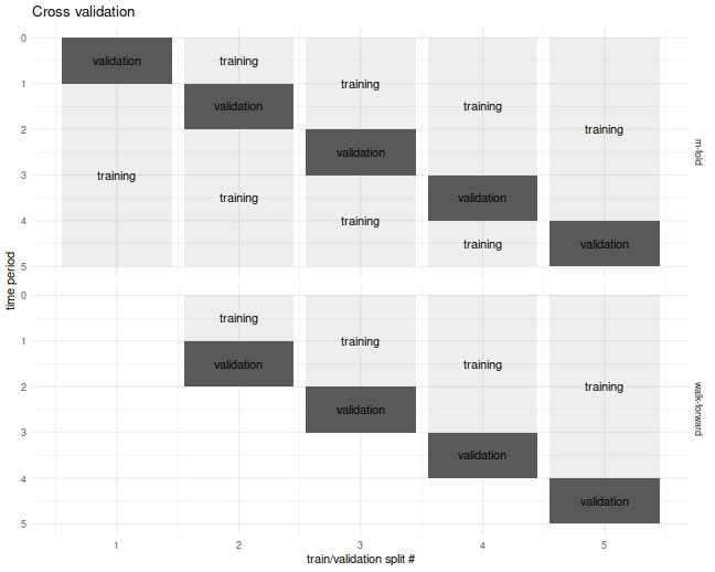
For the specific problem of estimating what I call the achieved signal-noise ratio of the Markowitz portfolio, one can use the Sharpe Ratio Information Criterion of Paulsen and Söhl. However, I suspect most practicing quants would fall back to cross validation. Cross validation is a folk remedy prescribed to cure all ills, probably beneficial but of unknown efficacy. In the usual \(m\) fold cross validation, one splits the data into \(m\) equally sized pieces, fits the Markowitz portfolio on all but one of those \(m\) pieces, then simulates returns on that piece. This is repeated holding out each of the \(m\) validation sets. The result is a simulated time series over the \(n\) days of data, which one then computes the Sharpe ratio on. I commonly used a fancier version of cross validation, called walk forward, where one only estimated the portfolio on data prior to the validation set, which results in a slightly truncated resultant time series. The \(m\)-fold and walk-forward cross validation techniques are illustrated below for the case of \(m=5\) folds.

Cross Validation is Broken?

Although I used cross-validation in this way for years, I never tested it until now. It seemed "obvious" that it would provide unbiased results. It turns out I was wrong, as simple simulations will show.

In our set up, cross validation is designed to estimate the achieved signal-noise ratio. "Achieved" means we are considering the signal-noise ratio of the sample Markowitz portfolio. This is a quantity that is both random (depends on the sample) and unobservable (depends on the population mean and covariance). In the simulations below I perform \(10\)-fold regular and walk-forward cross validation, constructing the Markowitz portfolio on training data, then generating a single time series of returns, computing the Sharpe on those returns. I also compute the achieved signal-noise ratio of the Markowitz portfolio on the whole sample. I vary the maximal signal-noise ratio of the population, as well as the number of assets. For every setting of the population parameters I perform 50000 simulations, then average the cross validated Sharpes and the achieved signal-noise ratios over the simulations.

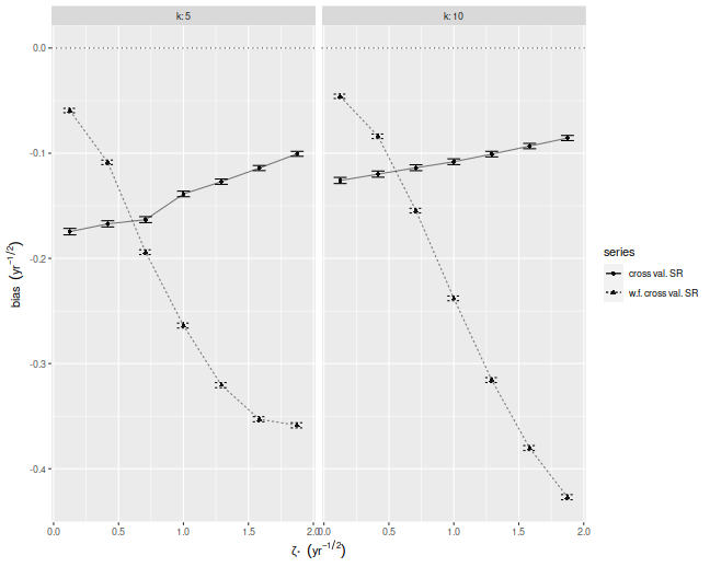
Below I plot the bias of the Sharpes estimated via regular and walk-forward cross validation, defined as the Sharpe minus the achieved signal-noise ratio. We see that, in annual terms, both cross validation techniques are severely biased, and walk-forward gets worse as the maximal signal-noise ratio increases. The bias is negative, which is to say we _under_estimate the achieved signal-noise ratio.

suppressMessages({
  library(dplyr)
  library(tidyr)
  library(tibble)
  library(future.apply)
})

# trading days per year
ope <- 252
# compute markowitz portfolio
comp_mp <- function(X) { solve(cov(X),colMeans(X)) }
# compute sr
comp_sr <- function(x,na.rm=TRUE) { mean(x,na.rm=na.rm) / sd(x,na.rm=na.rm) }
# run simulations
simit <- function(n,k,zeta,nsim=1000,nfolds=10) {
  require(future.apply)
  won <- seq(n)
  cvidx <- (won %% nfolds) + 1
  mu <- zeta / sqrt(k)
  vals <- future_replicate(nsim,{
    X <- matrix(rnorm(n*k,mean=mu),ncol=k)
    kfret <- rep(0,n)
    wfret <- rep(NA_real_,n)
    for (folnum in unique(cvidx)) { 
      oosi <- cvidx==folnum
      oos <- X[oosi,]
      iis <- X[!oosi,]
      mp <- comp_mp(iis)
      kfret[oosi] <- oos %*% mp
      # walk forward
      iisi <- cvidx < folnum
      if (any(iisi)) {
        iis <- X[iisi,]
        mp <- comp_mp(iis)
        wfret[oosi] <- oos %*% mp
      }
    }
    cv_sr <- comp_sr(kfret)
    wf_sr <- comp_sr(wfret,na.rm=TRUE)
    achieved_snr <- sum(mu * mp) / sqrt(sum(mp^2))
    c(cv_sr,wf_sr,achieved_snr,sqrt(ope)*mean(kfret),sd(kfret))
  })
  setNames(data.frame(sqrt(ope) * t(vals)),c('CV','walkforward','achieved','kf_mean','kf_sd'))
}

nday <- ope*5
nsim <- 50000

params <- crossing(tibble(zeta=seq(0.125,1.875,length.out=7)/sqrt(ope)),tibble(k=c(5,10)))

set.seed(1234)
plan(multiprocess)
resu <- params %>%
  group_by(zeta,k) %>%
    summarize(foo=list(simit(n=nday,k=k,zeta=zeta,nsim=nsim))) %>%
  ungroup() %>%
  unnest(foo)
plan(sequential)

# aggregate the results
mresu <- resu %>%
  tidyr::gather(key=series,value=value,-zeta,-k,-achieved) %>%
  mutate(bias=value - achieved) %>%
  group_by(zeta,k,series) %>%
    summarize(emp_bias=mean(bias),
              emp_sbias=sd(bias),
              count=n()) %>%
  ungroup() %>%
  mutate(emp_biase=emp_sbias / sqrt(count)) 

ph <- mresu %>%
  dplyr::filter(series %in% c('CV','walkforward')) %>%
  mutate(showser=case_when(series=='CV'  ~ 'cross val. SR',
                           series=='walkforward' ~ 'w.f. cross val. SR',
                           TRUE ~ 'error')) %>%
  ggplot(aes(sqrt(ope)*zeta,emp_bias,
             linetype=showser,
             group=interaction(k,showser))) +
  geom_hline(yintercept=0,linetype=3,alpha=0.8) + 
  geom_point(aes(shape=showser),alpha=0.9) +
  geom_errorbar(aes(ymin=emp_bias - emp_biase,ymax=emp_bias + emp_biase),width=0.1) + 
  geom_line(alpha=0.5) +
  facet_wrap(~k,labeller=label_both) +
  labs(x=expression(zeta['*']~~(yr^{-1/2})),
       y=expression(bias~~(yr^{-1/2})),
       shape='series',
       linetype='series')
print(ph)

Where is the bias?

Despite the relative simplicity of the simulations, I was convinced they contained a bug. How could cross-validation be so broken? I tried increasing the number of folds, which only made the problem worse! In my debugging I noticed that the estimate of the mean return of the Markowitz portfolio seemed unbiased. How can one have an unbiased estimate of the mean, but a biased estimate of the Sharpe ratio? The answer to that question is that the sample mean and sample standard deviation are not independent under cross validation.

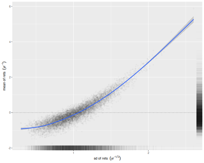
We illustrate that here by performing simulations where the population mean is the zero vector. For each simulation we compute the numerator and denominator of the cross-validated Sharpe ratio, namely the mean and standard deviation of the simulated returns on validation sets. We then scatter the means versus the standard deviations. There is a clear correlation here. I believe this is a well-known effect in cross-validation. Moreover, if your standard deviation is positively correlated with your mean, it will clearly bias your Sharpe ratio. This is simple to understand intuitively, we leave it as an exercise to show how that bias is a function of the correlation.

nday <- ope*5
nsim <- 10000

set.seed(1234)
plan(multiprocess)
atz <- simit(n=nday,k=5,zeta=0,nsim=nsim)
plan(sequential)

# scatter em
ph <- atz %>%
  ggplot(aes(kf_sd,kf_mean)) +
  geom_point(alpha=0.02) +
    stat_smooth() + 
    geom_hline(yintercept=0,linetype=3) + 
    geom_rug(alpha=0.02,sides='rb') + 
  labs(x=expression(sd~of~rets~~(yr^{-1/2})),
       y=expression(mean~of~rets~~(yr^{-1})))
print(ph)

What can be done?

If you intended to trade the Markowitz portfolio, you could probably debias the cross-validated estimates by some mathematical wizardry. However, most quants deploy more complicated trading strategies, which would be harder to analyze. My only suggestion at the moment is to instead use an average of Sharpes approach: perform cross-validation as usual, but instead of computing a single time series of returns, compute the Sharpe ratio on each validation set, then average them. In a future blog post I will show that this has far less bias for our toy problem.