Some of the research on the problem of "overfitting" of quantitative strategies
(including my own) might be better
described as research on "over-optimism". That is because the analysis
tends to view the strategies as something one stumbles upon, without any
in-sample tinkering. If that is the case, the Sharpe ratio is nearly
unbiased for the signal-noise ratio, and the only statistical sin is
selecting the best strategy among many without some kind of multiple hypothesis
test correction. However, strategies tend to be generated based on some
in-sample overfitting beyond just selection. As an example, suppose you
observed $n$ days of returns on $k$ assets in your universe, then constructed
the Markowitz portfolio based on that data. If your strategy is to hold
that Markowitz portfolio, it is a bit trickier to de-bias the in-sample Sharpe ratio.
For the specific problem of estimating what I call the achieved signal-noise
ratio of the Markowitz portfolio, one can use the Sharpe Ratio Information
Criterion of Paulsen and Söhl.
However, I suspect most practicing quants would fall back to cross validation.
Cross validation is a folk remedy
prescribed to cure all ills, probably beneficial but of unknown efficacy.
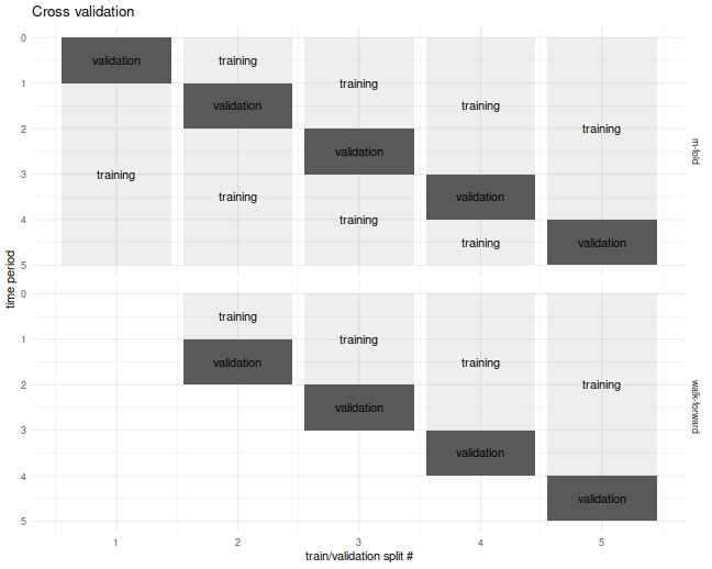
In the usual $m$ fold cross validation, one splits the data into $m$ equally
sized pieces, fits the Markowitz portfolio on all but one of those $m$ pieces,
then simulates returns on that piece. This is repeated holding out each of the $m$
validation sets. The result is a simulated time series over the $n$ days of
data, which one then computes the Sharpe ratio on.
I commonly used a fancier version of cross validation, called walk forward,
where one only estimated the portfolio on data prior to the validation set,
which results in a slightly truncated resultant time series.
The $m$-fold and walk-forward cross validation techniques are illustrated
below for the case of $m=5$ folds.
Cross Validation is Broken?
Although I used cross-validation in this way for years, I never tested it until now.
It seemed "obvious" that it would provide unbiased results.
It turns out I was wrong, as simple simulations will show.
In our set up, cross validation is designed to estimate the achieved
signal-noise ratio. "Achieved" means we are considering the signal-noise ratio
of the sample Markowitz portfolio. This is a quantity that is both random
(depends on the sample) and unobservable (depends on the population mean and
covariance).
In the simulations below I perform $10$-fold regular and walk-forward cross validation,
constructing the Markowitz portfolio on training data, then generating a single
time series of returns, computing the Sharpe on those returns.
I also compute the achieved signal-noise ratio of the Markowitz portfolio
on the whole sample.
I vary the maximal signal-noise ratio of the population, as well as the
number of assets.
For every setting of the population parameters I perform 50000 simulations,
then average the cross validated Sharpes and the achieved signal-noise
ratios over the simulations.
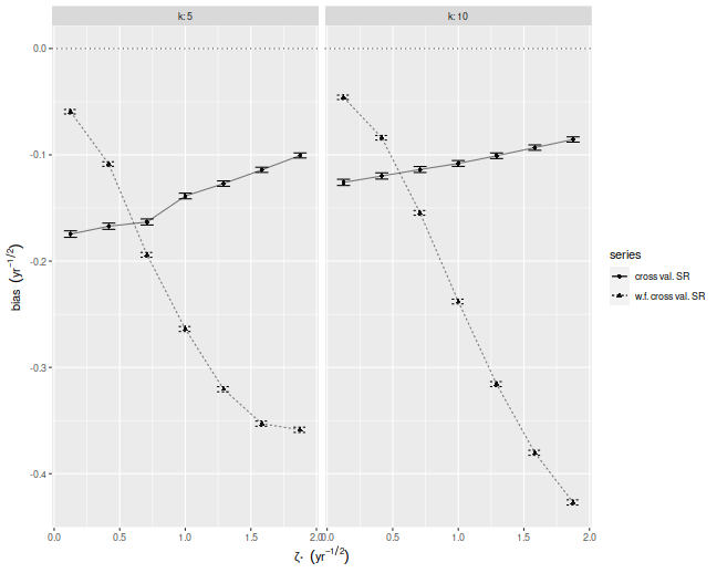
Below I plot the bias of the Sharpes estimated via regular and walk-forward
cross validation, defined as the Sharpe minus the achieved signal-noise ratio.
We see that, in annual terms, both cross validation techniques are severely
biased, and walk-forward gets worse as the maximal signal-noise ratio
increases. The bias is negative, which is to say we _under_estimate the
achieved signal-noise ratio.
suppressMessages({
  library(dplyr)
  library(tidyr)
  library(tibble)
  library(future.apply)
})

# trading days per year
ope <- 252
# compute markowitz portfolio
comp_mp <- function(X) { solve(cov(X),colMeans(X)) }
# compute sr
comp_sr <- function(x,na.rm=TRUE) { mean(x,na.rm=na.rm) / sd(x,na.rm=na.rm) }
# run simulations
simit <- function(n,k,zeta,nsim=1000,nfolds=10) {
  require(future.apply)
  won <- seq(n)
  cvidx <- (won %% nfolds) + 1
  mu <- zeta / sqrt(k)
  vals <- future_replicate(nsim,{
    X <- matrix(rnorm(n*k,mean=mu),ncol=k)
    kfret <- rep(0,n)
    wfret <- rep(NA_real_,n)
    for (folnum in unique(cvidx)) {
      oosi <- cvidx==folnum
      oos <- X[oosi,]
      iis <- X[!oosi,]
      mp <- comp_mp(iis)
      kfret[oosi] <- oos %*% mp
      # walk forward
      iisi <- cvidx < folnum
      if (any(iisi)) {
        iis <- X[iisi,]
        mp <- comp_mp(iis)
        wfret[oosi] <- oos %*% mp
      }
    }
    cv_sr <- comp_sr(kfret)
    wf_sr <- comp_sr(wfret,na.rm=TRUE)
    achieved_snr <- sum(mu * mp) / sqrt(sum(mp^2))
    c(cv_sr,wf_sr,achieved_snr,sqrt(ope)*mean(kfret),sd(kfret))
  })
  setNames(data.frame(sqrt(ope) * t(vals)),c('CV','walkforward','achieved','kf_mean','kf_sd'))
}

nday <- ope*5
nsim <- 50000

params <- crossing(tibble(zeta=seq(0.125,1.875,length.out=7)/sqrt(ope)),tibble(k=c(5,10)))

set.seed(1234)
plan(multicore)
resu <- params %>%
  group_by(zeta,k) %>%
    summarize(foo=list(simit(n=nday,k=k,zeta=zeta,nsim=nsim))) %>%
  ungroup() %>%
  unnest(foo)
plan(sequential)
# aggregate the results:
mresu <- resu %>%
  tidyr::gather(key=series,value=value,-zeta,-k,-achieved) %>%
  mutate(bias=value - achieved) %>%
  group_by(zeta,k,series) %>%
    summarize(emp_bias=mean(bias),
              emp_sbias=sd(bias),
              count=n()) %>%
  ungroup() %>%
  mutate(emp_biase=emp_sbias / sqrt(count))

ph <- mresu %>%
  dplyr::filter(series %in% c('CV','walkforward')) %>%
  mutate(showser=case_when(series=='CV'  ~ 'cross val. SR',
                           series=='walkforward' ~ 'w.f. cross val. SR',
                           TRUE ~ 'error')) %>%
  ggplot(aes(sqrt(ope)*zeta,emp_bias,
             linetype=showser,
             group=interaction(k,showser))) +
  geom_hline(yintercept=0,linetype=3,alpha=0.8) +
  geom_point(aes(shape=showser),alpha=0.9) +
  geom_errorbar(aes(ymin=emp_bias - emp_biase,ymax=emp_bias + emp_biase),width=0.1) +
  geom_line(alpha=0.5) +
  facet_wrap(~k,labeller=label_both) +
  labs(x=expression(zeta['*']~~(yr^{-1/2})),
       y=expression(bias~~(yr^{-1/2})),
       shape='series',
       linetype='series')
print(ph)
Where is the bias?
Despite the relative simplicity of the simulations, I was convinced they
contained a bug. How could cross-validation be so broken?
I tried increasing the number of folds, which only made the problem worse!
In my debugging I noticed that the estimate of the mean return of the
Markowitz portfolio seemed unbiased.
How can one have an unbiased estimate of the mean, but a biased estimate
of the Sharpe ratio?
The answer to that question is that the sample mean and sample standard
deviation are not independent under cross validation.
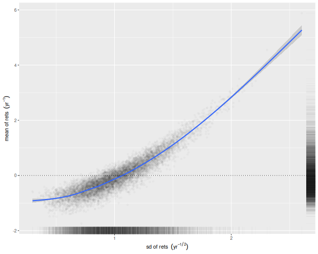
We illustrate that here by performing simulations where the population
mean is the zero vector. For each simulation we compute the numerator and
denominator of the cross-validated Sharpe ratio, namely the mean and
standard deviation of the simulated returns on validation sets.
We then scatter the means versus the standard deviations.
There is a clear correlation here.
I believe this is a well-known effect in cross-validation.
Moreover, if your standard deviation is positively correlated
with your mean, it will clearly bias your Sharpe ratio.
This is simple to understand intuitively, we
leave it as an exercise to show how that bias
is a function of the correlation.
nday <- ope*5
nsim <- 10000

set.seed(1234)
plan(multiprocess)
atz <- simit(n=nday,k=5,zeta=0,nsim=nsim)
plan(sequential)

# scatter em:
ph <- atz %>%
  ggplot(aes(kf_sd,kf_mean)) +
  geom_point(alpha=0.02) +
    stat_smooth() +
    geom_hline(yintercept=0,linetype=3) +
    geom_rug(alpha=0.02,sides='rb') +
  labs(x=expression(sd~of~rets~~(yr^{-1/2})),
       y=expression(mean~of~rets~~(yr^{-1})))
print(ph)
What can be done?
If you intended to trade the Markowitz portfolio, you could probably debias
the cross-validated estimates by some mathematical wizardry.
However, most quants deploy more complicated trading strategies,
which would be harder to analyze.
My only suggestion at the moment is to instead use an average of Sharpes
approach: perform cross-validation as usual, but instead of computing a single
time series of returns, compute the Sharpe ratio on each validation set,
then average them. In a future blog post I will show that this has far less
bias for our toy problem.
Click to read and post comments
Consider the following challenge:
estimate the Signal-Noise ratio of an asset given a single
observation of returns of that asset, $x$.
The task seems impossible: you can easily estimate the mean, but
how are you going to estimate the standard deviation
with just one observation?
Consider, however,
that for most assets the expected value of returns is very small compared to the volatility,
so if you wanted to estimate the variance of returns, $x^2$ would be a good guess.
Thus $\left|x\right|$ would be a passable estimate for the standard deviation.
Given that $x$ is an unbiased estimate of the mean, then
$$
\frac{x}{\left|x\right|} = \operatorname{sign}(x)
$$
is our candidate estimator of the Signal-Noise ratio.
It turns out this will work, up to scaling.
Suppose that returns are Gaussian. Then
$$
E\left[
\operatorname{sign}(x)
\right] = 2\Phi\left(\frac{\mu}{\sigma}\right) - 1
\approx \sqrt{\frac{2}{\pi}} \frac{\mu}{\sigma}.
$$
Thus $\sqrt{\frac{\pi}{2}} \operatorname{sign}(x)$
is a nearly unbiased estimator of the Signal-Noise ratio.
Since this estimator has only two possible values, it is going to be very noisy.
However, if you had $n$ observations $x_t$, you could
average them together as
$$
\check{\zeta} = \frac{1}{n}\sqrt{\frac{\pi}{2}} \sum_{1 \le t \le n}\operatorname{sign}\left(x_t\right).
$$
Call this the sign Sharpe ratio.
Note that it is just a rescaled version of the cringe-worthy "winning days percentage"
statistic some portfolio managers advertise.
There are two obvious problems with the sign Sharpe ratio.
- It is easy to show that the standard error of $\check{\zeta}$ is
$\sqrt{\frac{\pi}{2n}}$, which is about 20% bigger than that
of the moment-based Sharpe ratio.
- It is only nearly unbiased for Gaussian returns, and can have
serious bias for skewed returns.
The latter point is a serious problem. One can easily construct returns
streams with absurdly high or low values of winning days percentage,
and somewhat arbitrary signal-noise ratio.
By using the Edgeworth expansion, one can show that the expected value
of $\check{\zeta}$ is approximately
$$
E\left[
\check{\zeta}
\right] \approx \zeta - \frac{\gamma_1}{6},
$$
where $\zeta=\mu/\sigma$ is the Signal-Noise ratio, and $\gamma_1$ is the
standardized skewness of returns. Of course, if you somehow knew the skew
of returns, you could correct for them.
More interesting would be to find a way to estimate $\gamma_1$ from a
single observation, though I would argue that
$c\operatorname{sign}\left(x\right)$ is probably the best candidate.
Let's confirm these findings experimentally.
Consider the case where $x_t$ are drawn from a Beta distribution,
shifted to have a fixed mean.
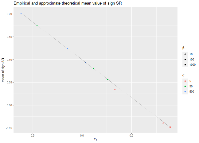
We fix the Signal-Noise ratio to be 0.1, and
tweak the two shape parameters of the Beta distribution,
$\alpha$ and $\beta$, to vary the skewness of returns.
We plot the empirical mean value of $\check{\zeta}$ for
$n=10^7$, along with the approximate theoretical value,
versus the skewness.
We see very good agreement between the two except for the case
where $\alpha$ and $\beta$ are small, where the higher order moments
which we have discarded are no longer negligible.
We would note that this is also likely to be a problem for
real world asset returns.
library(dplyr)
library(tidyr)
library(tibble)
library(ggplot2)

# generate shifted beta variates with a fixed SNR zeta
genb <- function(n,zeta,alpha,beta) {
  mu <- alpha / (alpha+beta)
  sg <- sqrt(alpha*beta/((alpha+beta+1)*(alpha+beta)^2))
  x <- (sg*zeta - mu) + rbeta(n,shape1=alpha,shape2=beta)
}
signsr <- function(x) { sqrt(pi/2) * mean(sign(x)) }

zeta <- 0.1
set.seed(12345)
sims <- crossing(tibble(alpha=c(5,50,500)),tibble(beta=c(10,100,1000))) %>%
  group_by(alpha,beta) %>%
    summarize(simzet=signsr(genb(n=10000000,zeta=zeta,alpha=alpha,beta=beta)),
              skew=2*(beta-alpha)*sqrt(beta+alpha+1)/((alpha+beta+2)*sqrt(alpha*beta))) %>%
  ungroup() %>%
  mutate(esign=zeta - skew / 6)

# plot them:
sims %>%
  ggplot(aes(skew,simzet)) +
  geom_point(aes(color=factor(alpha),shape=factor(beta))) +
  geom_line(aes(y=esign),linetype=3,alpha=0.5) +
  labs(x=expression(gamma[1]),
       y='mean of sign SR',
       title='Empirical and approximate theoretical mean value of sign SR',
       color=expression(alpha),shape=expression(beta))
Is it useful?
The sign Sharpe ratio does not seem useful for estimating the Signal-Noise
ratio: it is too noisy, and is confounded by higher order moments.
However, the challenge of estimating the Sharpe from individual
observations was motivated by difficulties bounding the out-of-sample
Sharpe ratio from the-in-sample Sharpe ratio using something
like VC dimension or Rademacher complexity. The problem is that
the standard deviation in the Sharpe computation depends on all the
observations. As a side effect, if you increase a single day's returns,
it can cause the Sharpe to either increase or decrease.
Because of this dependence on the whole sample,
the Sharpe ratio can not easily be analyzed by these complexity measures.
Click to read and post comments
Previously on this blog we had performed a fair amount of testing of the
"drawdown-based estimator" of the signal-noise ratio,
as proposed by Damien Challet.
All that analysis was based on the 1.1 version of the
sharpeRratio package,
written by Challet himself.
There was a bug (or bugs) in that package that caused the estimator to be biased,
which could also appear as improved efficiency over the traditional
"moment-based" estimator due to Sharpe (or Gosset, rather) via shrinkage to zero.
Here we analyze the 1.2 version of the package, which presumably fixes this
issue.
Checking for bias
Here I perform some simulations to check for bias of the estimator.
I draw 128 days of daily returns from a $t$
distribution with $\nu=4$ degrees of freedom.
I then compute: the moment-based Sharpe ratio;
the moment-based Sharpe ratio, but debiased using higher order moments;
the drawdown estimator from the 1.2 version of the package;
the drawdown estimator from the 1.2 version of the package, but feeding
$\nu$ to the estimator.
I do this for many draws of returns.
I repeat for 256 days of data,
and for the population Signal-Noise ratio varying from
0.30 to 1.5 in "annualized units" (per square root year), assuming
252 trading days per year.
I use future.apply to run the simulations in parallel.
suppressMessages({
  library(dplyr)
  library(tidyr)
  library(tibble)
  library(SharpeR)
  library(sharpeRratio)
  library(future.apply)
})
# only works for scalar pzeta:
onesim <- function(nday,pzeta=0.1,nu=4) {
  x <- pzeta + sqrt(1 - (2/nu)) * rt(nday,df=nu)
  srv <- SharpeR::as.sr(x,higher_order=TRUE)
  # mental note: this is much more awkward than it should be,
  # let's make it easier in SharpeR!
  #ssr <- mean(x) / sd(x)
  # moment based:
  ssr <- srv$sr
  # debiased
  ssr_b <- ssr - SharpeR::sr_bias(snr=ssr,n=nday,cumulants=srv$cumulants)

  sim <- sharpeRratio::estimateSNR(x)
  # this cheats and gives the true nu to the estimator
  cht <- sharpeRratio::estimateSNR(x,nu=nu)
  c(ssr,ssr_b,sim$SNR,cht$SNR)
}
repsim <- function(nrep,nday,pzeta=0.1,nu=4) {
  dummy <- invisible(capture.output(jumble <- replicate(nrep,onesim(nday=nday,pzeta=pzeta,nu=nu)),file='/dev/null'))
  retv <- t(jumble)
  colnames(retv) <- c('sr','sr_unbiased','ddown','ddown_cheat')
  invisible(as.data.frame(retv))
}
manysim <- function(nrep,nday,pzeta,nu=4,nnodes=5) {
  if (nrep > 2*nnodes) {
    # do in parallel.
    nper <- table(1 + ((0:(nrep-1) %% nnodes)))
    plan(multisession, workers = 2)
    retv <- future_lapply(nper,FUN=function(aper) repsim(aper,nday=nday,pzeta=pzeta,nu=nu)) %>%
      bind_rows()
    plan(sequential)
  } else {
    retv <- repsim(nrep=nrep,nday=nday,pzeta=pzeta,nu=nu)
  }
  retv
}
# summarizing function
sim_summary <- function(retv) {
  retv %>%
    tidyr::gather(key=metric,value=value,-pzeta,-nday) %>%
        dplyr::filter(!is.na(value)) %>%
    group_by(pzeta,nday,metric) %>%
    summarize(meanvalue=mean(value),
              serr=sd(value) / sqrt(n()),
              rmse=sqrt(mean((pzeta - value)^2)),
              nsims=n()) %>%
    ungroup() %>%
    arrange(pzeta,nday,metric)
}

ope <- 252
pzeta <- seq(0.30,1.5,by=0.30) / sqrt(ope)

params <- tidyr::crossing(tibble::tribble(~nday,128,256),
                          tibble::tibble(pzeta=pzeta))

nrep <- 1000
set.seed(1234)
system.time({
  results <- params %>%
    group_by(nday,pzeta) %>%
      summarize(sims=list(manysim(nrep=nrep,nnodes=7,pzeta=pzeta,nday=nday))) %>%
    ungroup() %>%
    tidyr::unnest(cols=c(sims))
})
   user  system elapsed
  3.926   0.165 217.285
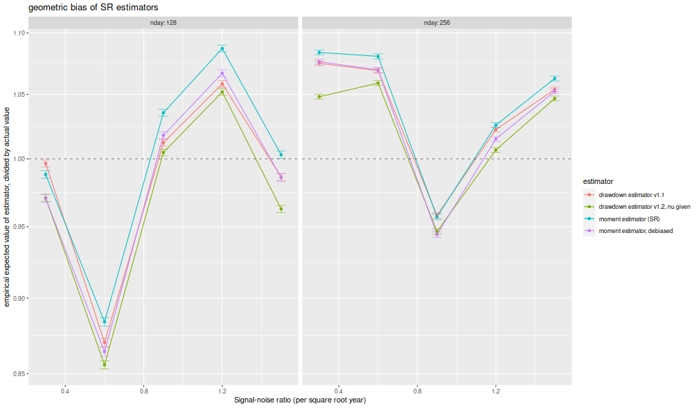
I compute the mean of each estimator over the 1,000 draws,
divide that mean estimate by the true Signal-Noise Ratio,
then plot versus the annualized SNR.
I plot errobars at plus and minus one standard error around the mean.
The ratio should be one, any deviation from which is geometric bias in the estimator.
Previously this plot showed the drawdown estimator consistently
estimating a value around 70% of the true value,
a problem which seems to have been fixed, as it
now shows values around 95% of the true value.
The moment estimator shows a slight positive
bias, which is decreasing in sample size, as described by Bao and Miller and Gehr.
The higher order moment correction mitigates this effect somewhat for the moment estimator.
library(ggplot2)
ph <- results %>%
  sim_summary() %>%
  mutate(metric=case_when(.$metric=='ddown' ~ 'drawdown estimator v1.1',
                          .$metric=='ddown_two' ~ 'drawdown estimator v1.2',
                          .$metric=='ddown_cheat' ~ 'drawdown estimator v1.2, nu given',
                          .$metric=='sr_unbiased' ~ 'moment estimator, debiased',
                          .$metric=='sr' ~ 'moment estimator (SR)',
                          TRUE ~ 'error')) %>%
  mutate(bias = meanvalue / pzeta,
         zeta_pa=sqrt(ope) * pzeta,
         serr = serr) %>%
  ggplot(aes(zeta_pa,bias,color=metric,ymin=bias-serr,ymax=bias+serr)) +
  geom_line() + geom_point() + geom_errorbar(alpha=0.5,width=0.05) +
  geom_hline(yintercept=1,linetype=2,alpha=0.5) +
  facet_wrap(~nday,labeller=label_both) +
  scale_y_log10() +
  labs(x='Signal-noise ratio (per square root year)',
       y='empirical expected value of estimator, divided by actual value',
       color='estimator',
       title='geometric bias of SR estimators')
print(ph)
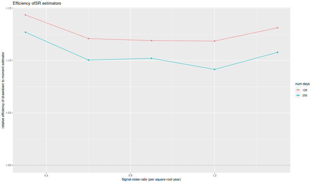
I now plot the 'relative efficiency' as in Figure 4 of version 6 of
Challet's paper.
This is the ratio of the mean square error of the moment-estimator
to the mean square error of the drawdown-estimator, again
as a function of the true (annualized) signal-noise ratio,
with different lines for the number of days simulated.
Challet's plot shows this line as approximately 5, while
we see values of around 1.25 or so.
That is, we see only modest improvements in efficiency for the
drawdown estimator, and not the putative huge gains in efficiency
in the paper.
library(ggplot2)
ph <- results %>%
  sim_summary() %>%
    dplyr::filter(metric %in% c('sr','ddown')) %>%
  dplyr::select(-meanvalue,-serr,-nsims) %>%
  tidyr::spread(key=metric,value=rmse) %>%
  mutate(eff=(sr/ddown)^2) %>%
  mutate(zeta_pa=sqrt(ope) * pzeta) %>%
  ggplot(aes(zeta_pa,eff,color=factor(nday))) +
  geom_line() + geom_point() +
  geom_hline(yintercept=1,linetype=3) +
  labs(x='Signal-noise ratio (per square root year)',
       y='relative efficiency of drawdown to moment estimator',
       color='num days',
       title='Efficiency of SR estimators')
print(ph)
Thus it appears that the 1.2 version of the package fixes
the bias issues in the initial release.
Click to read and post comments
In chapter 4 of our Short Sharpe Course,
we analyzed in great detail the standard error of the Sharpe ratio
under a number of deviations from the assumptions of i.i.d. normal returns.
By showing that the standard error does not differ too much from the nominal
value, we established that hypothesis testing with moderate type I error
rates is largely achievable.
However, these results do not necessarily support testing with very small type I
rates, as the tail distribution of the Sharpe ratio may be far from Gaussian.
It turns out
there are known bounds on large deviations of the $t$-statistic which
we can directly translate into equivalent facts regarding the Sharpe.
It is not surprising that one of these results was coauthored by Peter Hall,
who wrote a book on the convergence rates of the Central Limit Theorem.
Under the null hypothesis, $\zeta=0$,
Wang and Hall
showed that
$$
\mathcal{P}\left(\zeta \ge q\right) \approx \left(1 - \Phi\left(\frac{n}{n-1}\sqrt{n}q\right)\right)
\operatorname{exp}\left(-\frac{1}{3} \left(\frac{nq}{n-1}\right)^3 n \gamma_1 \right).
$$
Here $\gamma_1$ is the skewness of returns and
$\Phi\left(x\right)$ is the Gaussian distribution, and thus the approximation
(which holds up to a factor in $n^{-1}$)
compares the exceedance probability of the Sharpe ratio to the equivalent Gaussian law.
For moderately skewed returns and modestly sized $n$, we expect the
correction factor to be around $1\pm 0.1$ or so.
This means that the type I rate assuming a normal distribution for the
Sharpe is ``usually'' within 10% of nominal.
It is worth noting that the deviance from the normal approximation
is affected not by kurtosis per se, but by the skewness,
which is to be expected from the Berry-Esseen theorem.
We note that in the case $\zeta\ne0$, a more complicated version of the approximation holds,
but we defer this to our updated Short Sharpe Course.
Simulations
Here we confirm the relationship above empirically.
We draw returns from a
``Lambert W $\times$ Gaussian'' distribution, with
the skew parameter, $\delta$ varying from $-0.4$ to $0.4$,
and we set $n$ to 8 years of daily data.
For each setting of the skew we perform many simulations under
the null hypothesis, $\zeta=0$, then compute the empirical probability that the
Sharpe ratio exceeds some value $q$.
suppressMessages({
  library(dplyr)
  library(tidyr)
  library(magrittr)
  library(future.apply)
  library(LambertW)
  library(tibble)
    library(zipper) # remotes::install_github('shabbychef/zipper')
})
#Lambert x Gaussian
gen_lambert_w <- function(n,dl = 0.1,mu = 0,sg = 1) {
  require(LambertW,quietly=TRUE)
  suppressWarnings({
    Gauss_input = create_LambertW_input("normal", beta=c(0,1))
    params = list(delta = c(0), gamma=c(dl), alpha = 1)
    LW.Gauss = create_LambertW_output(Gauss_input, theta = params)
    #get the moments of this distribution
    moms <- mLambertW(beta=c(0,1),distname=c("normal"),delta = 0,gamma = dl, alpha = 1)
  })
  if (!is.null(LW.Gauss$r)) {
    # API changed in 0.5:
    samp <- LW.Gauss$r(n=n)
  } else {
    samp <- LW.Gauss$rY(params)(n=n)
  }
  samp <- mu  + (sg/moms$sd) * (samp - moms$mean)
}
moms_lambert_w <- function(dl = 0.1,mu = 0,sg = 1) {
  require(LambertW,quietly=TRUE)
  suppressWarnings({
    Gauss_input = create_LambertW_input("normal", beta=c(0,1))
    params = list(delta = c(0), gamma=c(dl), alpha = 1)
    LW.Gauss = create_LambertW_output(Gauss_input, theta = params)
    #get the moments of this distribution
    moms <- mLambertW(beta=c(0,1),distname=c("normal"),delta = 0,gamma = dl, alpha = 1)
  })
  moms$mean <- mu
  moms$sd <- sg
  return(moms)
}

# columnwise Sharpe
colsr <- function(X) { (colMeans(X) / apply(X,2,sd)) }
srsims <- function(nsim,nday,...) { colsr(matrix(gen_lambert_w(nsim*nday,...),nrow=nday)) }
manysims <- function(nsim,nday,dl=0.1,cuts=100) {
  require(future.apply)
  as.numeric(future_replicate(cuts,{ srsims(ceiling(nsim/cuts),nday=nday,dl=dl) }))
}
propex <- function(srs,vals=seq(0,0.5,length.out=301)) {
  require(zipper)  # install.github('shabbychef/zipper')
  places <- zipper::zip_le(sort(srs),vals)
  1 - (places + 0.5) / (length(srs) + 1)
}
exceedance <- function(nday,dl=0.1,nsim=1e4,vals=seq(0,0.5,length.out=301)) {
  srs <- manysims(nsim=nsim,nday=nday,dl=dl)
  ppp <- propex(srs=srs,vals=vals)
  moms <- moms_lambert_w(dl=dl)
  tibble(vals=vals,prop=ppp,skewness=moms$skewness)
}

params <- tidyr::crossing(tibble::tribble(~n,8*252),
                          tibble::tribble(~dl,-0.4,0,0.4))

# sims:
nsim <- 1e6
plan(multicore,workers=7)
set.seed(1234)
suppressMessages({
  resu <- params %>%
    group_by(n,dl) %>%
    summarize(sims=list(exceedance(nday=n,dl=dl,nsim=nsim))) %>%
    ungroup() %>%
    tidyr::unnest(cols=c(sims))
})
plan(sequential)
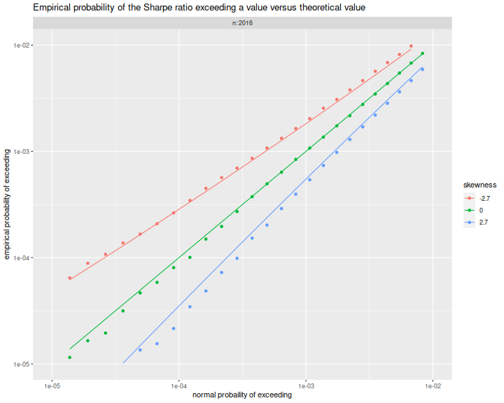
Here
we plot the empirical exceedance probabilities versus
$1 - \Phi\left(\frac{n}{n-1}\sqrt{n}q\right)$, with lines for the
right hand side of the approximation above.
We see that the approximation matches the experiments fairly well.
library(ggplot2)
ph <- resu %>%
  mutate(norm_law=pnorm(sqrt(n)*(n/(n-1))*vals,lower.tail=FALSE)) %>%
  mutate(hall_law=norm_law * exp(-(1/3)*((n*vals/(n-1))^3) * n * skewness)) %>%
  mutate(fskew=factor(signif(skewness,2))) %>%
  ggplot(aes(norm_law,prop,color=fskew,group=interaction(n,dl))) +
  geom_point() +
  geom_line(aes(y=hall_law))+
  scale_x_log10(limits=c(1e-5,0.01)) +
  scale_y_log10(limits=c(1e-5,0.01)) +
  facet_wrap(~n,labeller=label_both) +
  labs(x='normal probability of exceeding',
       y='empirical probability of exceeding',
       color='skewness',
       title='Empirical probability of the Sharpe ratio exceeding a value versus theoretical value')
print(ph)
Click to read and post comments