Probability of large deviation of the Sharpe ratio
In chapter 4 of our Short Sharpe Course, we analyzed in great detail the standard error of the Sharpe ratio under a number of deviations from the assumptions of i.i.d. normal returns. By showing that the standard error does not differ too much from the nominal value, we established that hypothesis testing with moderate type I error rates is largely achievable. However, these results do not necessarily support testing with very small type I rates, as the tail distribution of the Sharpe ratio may be far from Gaussian.
It turns out there are known bounds on large deviations of the $t$-statistic which we can directly translate into equivalent facts regarding the Sharpe. It is not surprising that one of these results was coauthored by Peter Hall, who wrote a book on the convergence rates of the Central Limit Theorem. Under the null hypothesis, $\zeta=0$, Wang and Hall showed that $$ \mathcal{P}\left(\zeta \ge q\right) \approx \left(1 - \Phi\left(\frac{n}{n-1}\sqrt{n}q\right)\right) \operatorname{exp}\left(-\frac{1}{3} \left(\frac{nq}{n-1}\right)^3 n \gamma_1 \right). $$ Here $\gamma_1$ is the skewness of returns and $\Phi\left(x\right)$ is the Gaussian distribution, and thus the approximation (which holds up to a factor in $n^{-1}$) compares the exceedance probability of the Sharpe ratio to the equivalent Gaussian law. For moderately skewed returns and modestly sized $n$, we expect the correction factor to be around $1\pm 0.1$ or so. This means that the type I rate assuming a normal distribution for the Sharpe is ``usually'' within 10% of nominal.
It is worth noting that the deviance from the normal approximation is affected not by kurtosis per se, but by the skewness, which is to be expected from the Berry-Esseen theorem. We note that in the case $\zeta\ne0$, a more complicated version of the approximation holds, but we defer this to our updated Short Sharpe Course.
Simulations
Here we confirm the relationship above empirically. We draw returns from a ``Lambert W $\times$ Gaussian'' distribution, with the skew parameter, $\delta$ varying from $-0.4$ to $0.4$, and we set $n$ to 8 years of daily data. For each setting of the skew we perform many simulations under the null hypothesis, $\zeta=0$, then compute the empirical probability that the Sharpe ratio exceeds some value $q$.
suppressMessages({
  library(dplyr)
  library(tidyr)
  library(magrittr)
  library(future.apply)
  library(LambertW)
  library(tibble)
    library(zipper) # remotes::install_github('shabbychef/zipper')
})
#Lambert x Gaussian
gen_lambert_w <- function(n,dl = 0.1,mu = 0,sg = 1) {
  require(LambertW,quietly=TRUE)
  suppressWarnings({
    Gauss_input = create_LambertW_input("normal", beta=c(0,1))
    params = list(delta = c(0), gamma=c(dl), alpha = 1)
    LW.Gauss = create_LambertW_output(Gauss_input, theta = params)
    #get the moments of this distribution
    moms <- mLambertW(beta=c(0,1),distname=c("normal"),delta = 0,gamma = dl, alpha = 1)
  })
  if (!is.null(LW.Gauss$r)) {
    # API changed in 0.5:
    samp <- LW.Gauss$r(n=n)
  } else {
    samp <- LW.Gauss$rY(params)(n=n)
  }
  samp <- mu  + (sg/moms$sd) * (samp - moms$mean)
}
moms_lambert_w <- function(dl = 0.1,mu = 0,sg = 1) {
  require(LambertW,quietly=TRUE)
  suppressWarnings({
    Gauss_input = create_LambertW_input("normal", beta=c(0,1))
    params = list(delta = c(0), gamma=c(dl), alpha = 1)
    LW.Gauss = create_LambertW_output(Gauss_input, theta = params)
    #get the moments of this distribution
    moms <- mLambertW(beta=c(0,1),distname=c("normal"),delta = 0,gamma = dl, alpha = 1)
  })
  moms$mean <- mu
  moms$sd <- sg
  return(moms)
}

# columnwise Sharpe
colsr <- function(X) { (colMeans(X) / apply(X,2,sd)) }
srsims <- function(nsim,nday,...) { colsr(matrix(gen_lambert_w(nsim*nday,...),nrow=nday)) }
manysims <- function(nsim,nday,dl=0.1,cuts=100) {
  require(future.apply)
  as.numeric(future_replicate(cuts,{ srsims(ceiling(nsim/cuts),nday=nday,dl=dl) }))
}
propex <- function(srs,vals=seq(0,0.5,length.out=301)) {
  require(zipper)  # install.github('shabbychef/zipper')
  places <- zipper::zip_le(sort(srs),vals)
  1 - (places + 0.5) / (length(srs) + 1)
}
exceedance <- function(nday,dl=0.1,nsim=1e4,vals=seq(0,0.5,length.out=301)) {
  srs <- manysims(nsim=nsim,nday=nday,dl=dl)
  ppp <- propex(srs=srs,vals=vals)
  moms <- moms_lambert_w(dl=dl)
  tibble(vals=vals,prop=ppp,skewness=moms$skewness)
}

params <- tidyr::crossing(tibble::tribble(~n,8*252),
                          tibble::tribble(~dl,-0.4,0,0.4))

# sims:
nsim <- 1e6
plan(multicore,workers=7)
set.seed(1234)
suppressMessages({
  resu <- params %>%
    group_by(n,dl) %>%
    summarize(sims=list(exceedance(nday=n,dl=dl,nsim=nsim))) %>%
    ungroup() %>%
    tidyr::unnest(cols=c(sims))
})
plan(sequential)
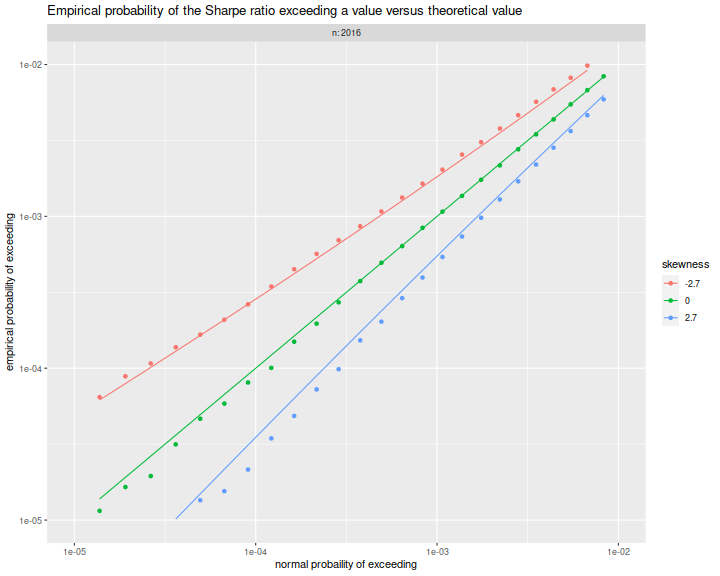
Here we plot the empirical exceedance probabilities versus $1 - \Phi\left(\frac{n}{n-1}\sqrt{n}q\right)$, with lines for the right hand side of the approximation above. We see that the approximation matches the experiments fairly well.
library(ggplot2)
ph <- resu %>%
  mutate(norm_law=pnorm(sqrt(n)*(n/(n-1))*vals,lower.tail=FALSE)) %>%
  mutate(hall_law=norm_law * exp(-(1/3)*((n*vals/(n-1))^3) * n * skewness)) %>%
  mutate(fskew=factor(signif(skewness,2))) %>%
  ggplot(aes(norm_law,prop,color=fskew,group=interaction(n,dl))) +
  geom_point() +
  geom_line(aes(y=hall_law))+
  scale_x_log10(limits=c(1e-5,0.01)) +
  scale_y_log10(limits=c(1e-5,0.01)) +
  facet_wrap(~n,labeller=label_both) +
  labs(x='normal probability of exceeding',
       y='empirical probability of exceeding',
       color='skewness',
       title='Empirical probability of the Sharpe ratio exceeding a value versus theoretical value')
print(ph)