A Sharper Sharpe, Again
Previously on this blog we had performed a fair amount of testing of the "drawdown-based estimator" of the signal-noise ratio, as proposed by Damien Challet. All that analysis was based on the 1.1 version of the sharpeRratio package, written by Challet himself. There was a bug (or bugs) in that package that caused the estimator to be biased, which could also appear as improved efficiency over the traditional "moment-based" estimator due to Sharpe (or Gosset, rather) via shrinkage to zero. Here we analyze the 1.2 version of the package, which presumably fixes this issue.
Checking for bias
Here I perform some simulations to check for bias of the estimator.
I draw 128 days of daily returns from a $t$
distribution with $\nu=4$ degrees of freedom.
I then compute: the moment-based Sharpe ratio;
the moment-based Sharpe ratio, but debiased using higher order moments;
the drawdown estimator from the 1.2 version of the package;
the drawdown estimator from the 1.2 version of the package, but feeding
$\nu$ to the estimator.
I do this for many draws of returns.
I repeat for 256 days of data,
and for the population Signal-Noise ratio varying from
0.30 to 1.5 in "annualized units" (per square root year), assuming
252 trading days per year.
I use future.apply to run the simulations in parallel.
suppressMessages({
  library(dplyr)
  library(tidyr)
  library(tibble)
  library(SharpeR)
  library(sharpeRratio)
  library(future.apply)
})
# only works for scalar pzeta:
onesim <- function(nday,pzeta=0.1,nu=4) {
  x <- pzeta + sqrt(1 - (2/nu)) * rt(nday,df=nu)
  srv <- SharpeR::as.sr(x,higher_order=TRUE)
  # mental note: this is much more awkward than it should be,
  # let's make it easier in SharpeR!
  #ssr <- mean(x) / sd(x)
  # moment based:
  ssr <- srv$sr
  # debiased
  ssr_b <- ssr - SharpeR::sr_bias(snr=ssr,n=nday,cumulants=srv$cumulants)

  sim <- sharpeRratio::estimateSNR(x)
  # this cheats and gives the true nu to the estimator
  cht <- sharpeRratio::estimateSNR(x,nu=nu)
  c(ssr,ssr_b,sim$SNR,cht$SNR)
}
repsim <- function(nrep,nday,pzeta=0.1,nu=4) {
  dummy <- invisible(capture.output(jumble <- replicate(nrep,onesim(nday=nday,pzeta=pzeta,nu=nu)),file='/dev/null'))
  retv <- t(jumble)
  colnames(retv) <- c('sr','sr_unbiased','ddown','ddown_cheat')
  invisible(as.data.frame(retv))
}
manysim <- function(nrep,nday,pzeta,nu=4,nnodes=5) {
  if (nrep > 2*nnodes) {
    # do in parallel.
    nper <- table(1 + ((0:(nrep-1) %% nnodes)))
    plan(multisession, workers = 2)
    retv <- future_lapply(nper,FUN=function(aper) repsim(aper,nday=nday,pzeta=pzeta,nu=nu)) %>%
      bind_rows()
    plan(sequential)
  } else {
    retv <- repsim(nrep=nrep,nday=nday,pzeta=pzeta,nu=nu)
  }
  retv
}
# summarizing function
sim_summary <- function(retv) {
  retv %>%
    tidyr::gather(key=metric,value=value,-pzeta,-nday) %>%
        dplyr::filter(!is.na(value)) %>%
    group_by(pzeta,nday,metric) %>%
    summarize(meanvalue=mean(value),
              serr=sd(value) / sqrt(n()),
              rmse=sqrt(mean((pzeta - value)^2)),
              nsims=n()) %>%
    ungroup() %>%
    arrange(pzeta,nday,metric)
}

ope <- 252
pzeta <- seq(0.30,1.5,by=0.30) / sqrt(ope)

params <- tidyr::crossing(tibble::tribble(~nday,128,256),
                          tibble::tibble(pzeta=pzeta))

nrep <- 1000
set.seed(1234)
system.time({
  results <- params %>%
    group_by(nday,pzeta) %>%
      summarize(sims=list(manysim(nrep=nrep,nnodes=7,pzeta=pzeta,nday=nday))) %>%
    ungroup() %>%
    tidyr::unnest(cols=c(sims))
})
   user  system elapsed
  3.926   0.165 217.285
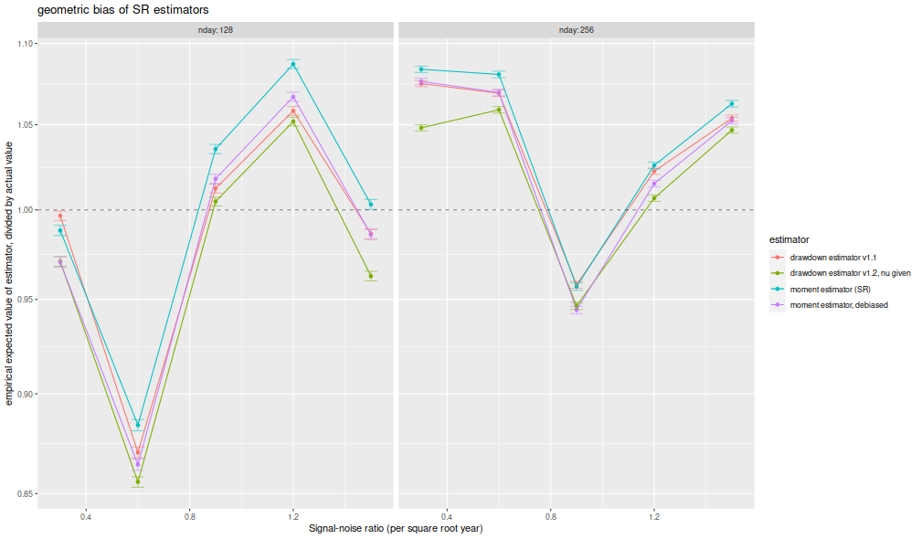
I compute the mean of each estimator over the 1,000 draws, divide that mean estimate by the true Signal-Noise Ratio, then plot versus the annualized SNR. I plot errobars at plus and minus one standard error around the mean. The ratio should be one, any deviation from which is geometric bias in the estimator. Previously this plot showed the drawdown estimator consistently estimating a value around 70% of the true value, a problem which seems to have been fixed, as it now shows values around 95% of the true value. The moment estimator shows a slight positive bias, which is decreasing in sample size, as described by Bao and Miller and Gehr. The higher order moment correction mitigates this effect somewhat for the moment estimator.
library(ggplot2)
ph <- results %>%
  sim_summary() %>%
  mutate(metric=case_when(.$metric=='ddown' ~ 'drawdown estimator v1.1',
                          .$metric=='ddown_two' ~ 'drawdown estimator v1.2',
                          .$metric=='ddown_cheat' ~ 'drawdown estimator v1.2, nu given',
                          .$metric=='sr_unbiased' ~ 'moment estimator, debiased',
                          .$metric=='sr' ~ 'moment estimator (SR)',
                          TRUE ~ 'error')) %>%
  mutate(bias = meanvalue / pzeta,
         zeta_pa=sqrt(ope) * pzeta,
         serr = serr) %>%
  ggplot(aes(zeta_pa,bias,color=metric,ymin=bias-serr,ymax=bias+serr)) +
  geom_line() + geom_point() + geom_errorbar(alpha=0.5,width=0.05) +
  geom_hline(yintercept=1,linetype=2,alpha=0.5) +
  facet_wrap(~nday,labeller=label_both) +
  scale_y_log10() +
  labs(x='Signal-noise ratio (per square root year)',
       y='empirical expected value of estimator, divided by actual value',
       color='estimator',
       title='geometric bias of SR estimators')
print(ph)
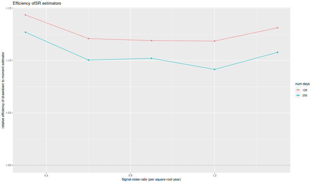
I now plot the 'relative efficiency' as in Figure 4 of version 6 of Challet's paper. This is the ratio of the mean square error of the moment-estimator to the mean square error of the drawdown-estimator, again as a function of the true (annualized) signal-noise ratio, with different lines for the number of days simulated. Challet's plot shows this line as approximately 5, while we see values of around 1.25 or so. That is, we see only modest improvements in efficiency for the drawdown estimator, and not the putative huge gains in efficiency in the paper.
library(ggplot2)
ph <- results %>%
  sim_summary() %>%
    dplyr::filter(metric %in% c('sr','ddown')) %>%
  dplyr::select(-meanvalue,-serr,-nsims) %>%
  tidyr::spread(key=metric,value=rmse) %>%
  mutate(eff=(sr/ddown)^2) %>%
  mutate(zeta_pa=sqrt(ope) * pzeta) %>%
  ggplot(aes(zeta_pa,eff,color=factor(nday))) +
  geom_line() + geom_point() +
  geom_hline(yintercept=1,linetype=3) +
  labs(x='Signal-noise ratio (per square root year)',
       y='relative efficiency of drawdown to moment estimator',
       color='num days',
       title='Efficiency of SR estimators')
print(ph)
Thus it appears that the 1.2 version of the package fixes the bias issues in the initial release.