Sharpe Ratio

A Sign Sharpe

Consider the following challenge: estimate the Signal-Noise ratio of an asset given a single observation of returns of that asset, \(x\). The task seems impossible: you can easily estimate the mean, but how are you going to estimate the standard deviation with just one observation? Consider, however, that for most assets the expected value of returns is very small compared to the volatility, so if you wanted to estimate the variance of returns, \(x^2\) would be a good guess. Thus \(\left|x\right|\) would be a passable estimate for the standard deviation. Given that \(x\) is an unbiased estimate of the mean, then

is our candidate estimator of the Signal-Noise ratio.

It turns out this will work, up to scaling. Suppose that returns are Gaussian. Then

Thus \(\sqrt{\frac{\pi}{2}} \operatorname{sign}(x)\) is a nearly unbiased estimator of the Signal-Noise ratio.

Since this estimator has only two possible values, it is going to be very noisy. However, if you had \(n\) observations \(x_t\), you could average them together as

Call this the sign Sharpe ratio. Note that it is just a rescaled version of the cringe-worthy "winning days percentage" statistic some portfolio managers advertise.

There are two obvious problems with the sign Sharpe ratio.

1. It is easy to show that the standard error of \(\check{\zeta}\) is \(\sqrt{\frac{\pi}{2n}}\), which is about 20% bigger than that of the moment-based Sharpe ratio.
2. It is only nearly unbiased for Gaussian returns, and can have serious bias for skewed returns.

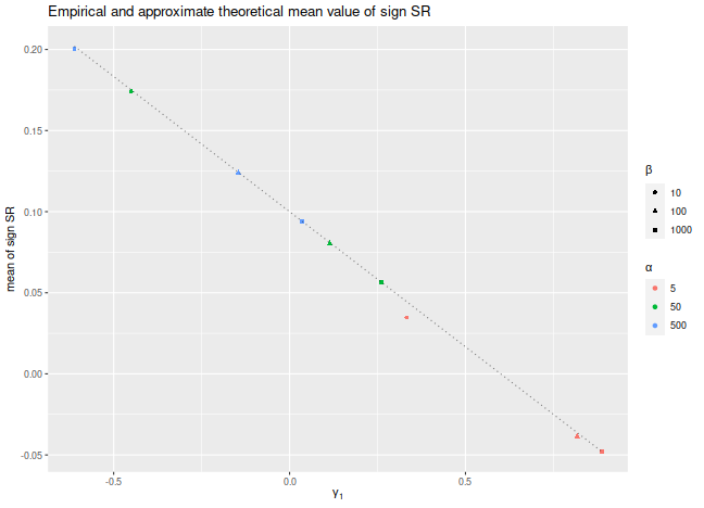
The latter point is a serious problem. One can easily construct returns streams with absurdly high or low values of winning days percentage, and somewhat arbitrary signal-noise ratio. By using the Edgeworth expansion, one can show that the expected value of \(\check{\zeta}\) is approximately

where \(\zeta=\mu/\sigma\) is the Signal-Noise ratio, and \(\gamma_1\) is the standardized skewness of returns. Of course, if you somehow knew the skew of returns, you could correct for them. More interesting would be to find a way to estimate \(\gamma_1\) from a single observation, though I would argue that \(c\operatorname{sign}\left(x\right)\) is probably the best candidate.

Let's confirm these findings experimentally. Consider the case where \(x_t\) are drawn from a Beta distribution, shifted to have a fixed mean. We fix the Signal-Noise ratio to be 0.1, and tweak the two shape parameters of the Beta distribution, \(\alpha\) and \(\beta\), to vary the skewness of returns. We plot the empirical mean value of \(\check{\zeta}\) for \(n=10^7\), along with the approximate theoretical value, versus the skewness. We see very good agreement between the two except for the case where \(\alpha\) and \(\beta\) are small, where the higher order moments which we have discarded are no longer negligible. We would note that this is also likely to be a problem for real world asset returns.

library(dplyr)
library(tidyr)
library(tibble)
library(ggplot2)

# generate shifted beta variates with a fixed SNR zeta
genb <- function(n,zeta,alpha,beta) {
  mu <- alpha / (alpha+beta)
  sg <- sqrt(alpha*beta/((alpha+beta+1)*(alpha+beta)^2))
  x <- (sg*zeta - mu) + rbeta(n,shape1=alpha,shape2=beta)
}
signsr <- function(x) { sqrt(pi/2) * mean(sign(x)) }

zeta <- 0.1
set.seed(12345)
sims <- crossing(tibble(alpha=c(5,50,500)),tibble(beta=c(10,100,1000))) %>%
  group_by(alpha,beta) %>%
    summarize(simzet=signsr(genb(n=10000000,zeta=zeta,alpha=alpha,beta=beta)),
              skew=2*(beta-alpha)*sqrt(beta+alpha+1)/((alpha+beta+2)*sqrt(alpha*beta))) %>%
  ungroup() %>%
  mutate(esign=zeta - skew / 6)

# plot them
sims %>%
  ggplot(aes(skew,simzet)) + 
  geom_point(aes(color=factor(alpha),shape=factor(beta))) + 
  geom_line(aes(y=esign),linetype=3,alpha=0.5) +
  labs(x=expression(gamma[1]),
       y='mean of sign SR',
       title='Empirical and approximate theoretical mean value of sign SR',
       color=expression(alpha),shape=expression(beta))

Is it useful?

The sign Sharpe ratio does not seem useful for estimating the Signal-Noise ratio: it is too noisy, and is confounded by higher order moments. However, the challenge of estimating the Sharpe from individual observations was motivated by difficulties bounding the out-of-sample Sharpe ratio from the-in-sample Sharpe ratio using something like VC dimension or Rademacher complexity. The problem is that the standard deviation in the Sharpe computation depends on all the observations. As a side effect, if you increase a single day's returns, it can cause the Sharpe to either increase or decrease. Because of this dependence on the whole sample, the Sharpe ratio can not easily be analyzed by these complexity measures.