Sharpe Ratio

A Sharper Sharpe, Again

Previously on this blog we had performed a fair amount of testing of the "drawdown-based estimator" of the signal-noise ratio, as proposed by Damien Challet. All that analysis was based on the 1.1 version of the sharpeRratio package, written by Challet himself. There was a bug (or bugs) in that package that caused the estimator to be biased, which could also appear as improved efficiency over the traditional "moment-based" estimator due to Sharpe (or Gosset, rather) via shrinkage to zero. Here we analyze the 1.2 version of the package, which presumably fixes this issue.

Checking for bias

Here I perform some simulations to check for bias of the estimator. I draw 128 days of daily returns from a $t$ distribution with $\nu=4$ degrees of freedom. I then compute: the moment-based Sharpe ratio; the moment-based Sharpe ratio, but debiased using higher order moments; the drawdown estimator from the 1.2 version of the package; the drawdown estimator from the 1.2 version of the package, but feeding $\nu$ to the estimator. I do this for many draws of returns. I repeat for 256 days of data, and for the population Signal-Noise ratio varying from 0.30 to 1.5 in "annualized units" (per square root year), assuming 252 trading days per year. I use future.apply to run the simulations in parallel.

suppressMessages({
  library(dplyr)
  library(tidyr)
  library(tibble)
  library(SharpeR)
  library(sharpeRratio)
  library(future.apply)
})
# only works for scalar pzeta:
onesim <- function(nday,pzeta=0.1,nu=4) {
  x <- pzeta + sqrt(1 - (2/nu)) * rt(nday,df=nu)
  srv <- SharpeR::as.sr(x,higher_order=TRUE)
  # mental note: this is much more awkward than it should be,
  # let's make it easier in SharpeR!
  #ssr <- mean(x) / sd(x)
  # moment based:
  ssr <- srv$sr
  # debiased
  ssr_b <- ssr - SharpeR::sr_bias(snr=ssr,n=nday,cumulants=srv$cumulants)

  sim <- sharpeRratio::estimateSNR(x)
  # this cheats and gives the true nu to the estimator
  cht <- sharpeRratio::estimateSNR(x,nu=nu)
  c(ssr,ssr_b,sim$SNR,cht$SNR)
}
repsim <- function(nrep,nday,pzeta=0.1,nu=4) {
  dummy <- invisible(capture.output(jumble <- replicate(nrep,onesim(nday=nday,pzeta=pzeta,nu=nu)),file='/dev/null'))
  retv <- t(jumble)
  colnames(retv) <- c('sr','sr_unbiased','ddown','ddown_cheat')
  invisible(as.data.frame(retv))
}
manysim <- function(nrep,nday,pzeta,nu=4,nnodes=5) {
  if (nrep > 2*nnodes) {
    # do in parallel.
    nper <- table(1 + ((0:(nrep-1) %% nnodes))) 
    plan(multisession, workers = 2)  
    retv <- future_lapply(nper,FUN=function(aper) repsim(aper,nday=nday,pzeta=pzeta,nu=nu)) %>%
      bind_rows()
    plan(sequential)
  } else {
    retv <- repsim(nrep=nrep,nday=nday,pzeta=pzeta,nu=nu)
  }
  retv 
}
# summarizing function
sim_summary <- function(retv) {
  retv %>%
    tidyr::gather(key=metric,value=value,-pzeta,-nday) %>%
        dplyr::filter(!is.na(value)) %>%
    group_by(pzeta,nday,metric) %>%
    summarize(meanvalue=mean(value),
              serr=sd(value) / sqrt(n()),
              rmse=sqrt(mean((pzeta - value)^2)),
              nsims=n()) %>%
    ungroup() %>%
    arrange(pzeta,nday,metric)
}

ope <- 252
pzeta <- seq(0.30,1.5,by=0.30) / sqrt(ope)

params <- tidyr::crossing(tibble::tribble(~nday,128,256),
                          tibble::tibble(pzeta=pzeta))

nrep <- 1000
set.seed(1234)
system.time({
  results <- params %>%
    group_by(nday,pzeta) %>%
      summarize(sims=list(manysim(nrep=nrep,nnodes=7,pzeta=pzeta,nday=nday))) %>%
    ungroup() %>%
    tidyr::unnest(cols=c(sims))
})

   user  system elapsed 
  3.926   0.165 217.285 

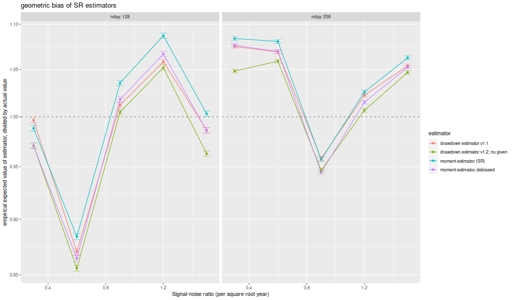
I compute the mean of each estimator over the 1,000 draws, divide that mean estimate by the true Signal-Noise Ratio, then plot versus the annualized SNR. I plot errobars at plus and minus one standard error around the mean. The ratio should be one, any deviation from which is geometric bias in the estimator. Previously this plot showed the drawdown estimator consistently estimating a value around 70% of the true value, a problem which seems to have been fixed, as it now shows values around 95% of the true value. The moment estimator shows a slight positive bias, which is decreasing in sample size, as described by Bao and Miller and Gehr. The higher order moment correction mitigates this effect somewhat for the moment estimator.

library(ggplot2)
ph <- results %>% 
  sim_summary() %>%
  mutate(metric=case_when(.$metric=='ddown' ~ 'drawdown estimator v1.1',
                          .$metric=='ddown_two' ~ 'drawdown estimator v1.2',
                          .$metric=='ddown_cheat' ~ 'drawdown estimator v1.2, nu given',
                          .$metric=='sr_unbiased' ~ 'moment estimator, debiased',
                          .$metric=='sr' ~ 'moment estimator (SR)',
                          TRUE ~ 'error')) %>%
  mutate(bias = meanvalue / pzeta,
         zeta_pa=sqrt(ope) * pzeta,
         serr = serr) %>%
  ggplot(aes(zeta_pa,bias,color=metric,ymin=bias-serr,ymax=bias+serr)) + 
  geom_line() + geom_point() + geom_errorbar(alpha=0.5,width=0.05) + 
  geom_hline(yintercept=1,linetype=2,alpha=0.5) + 
  facet_wrap(~nday,labeller=label_both) +
  scale_y_log10() + 
  labs(x='Signal-noise ratio (per square root year)',
       y='empirical expected value of estimator, divided by actual value',
       color='estimator',
       title='geometric bias of SR estimators')
print(ph)

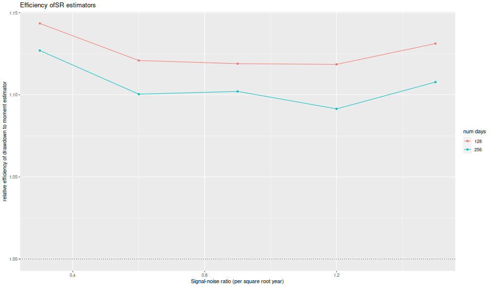
I now plot the 'relative efficiency' as in Figure 4 of version 6 of Challet's paper. This is the ratio of the mean square error of the moment-estimator to the mean square error of the drawdown-estimator, again as a function of the true (annualized) signal-noise ratio, with different lines for the number of days simulated. Challet's plot shows this line as approximately 5, while we see values of around 1.25 or so. That is, we see only modest improvements in efficiency for the drawdown estimator, and not the putative huge gains in efficiency in the paper.

library(ggplot2)
ph <- results %>% 
  sim_summary() %>%
    dplyr::filter(metric %in% c('sr','ddown')) %>%
  dplyr::select(-meanvalue,-serr,-nsims) %>%
  tidyr::spread(key=metric,value=rmse) %>%
  mutate(eff=(sr/ddown)^2) %>%
  mutate(zeta_pa=sqrt(ope) * pzeta) %>%
  ggplot(aes(zeta_pa,eff,color=factor(nday))) + 
  geom_line() + geom_point() + 
  geom_hline(yintercept=1,linetype=3) + 
  labs(x='Signal-noise ratio (per square root year)',
       y='relative efficiency of drawdown to moment estimator',
       color='num days',
       title='Efficiency of SR estimators')
print(ph)

Thus it appears that the 1.2 version of the package fixes the bias issues in the initial release.

Probability of large deviation of the Sharpe ratio

In chapter 4 of our Short Sharpe Course, we analyzed in great detail the standard error of the Sharpe ratio under a number of deviations from the assumptions of i.i.d. normal returns. By showing that the standard error does not differ too much from the nominal value, we established that hypothesis testing with moderate type I error rates is largely achievable. However, these results do not necessarily support testing with very small type I rates, as the tail distribution of the Sharpe ratio may be far from Gaussian.

It turns out there are known bounds on large deviations of the $t$-statistic which we can directly translate into equivalent facts regarding the Sharpe. It is not surprising that one of these results was coauthored by Peter Hall, who wrote a book on the convergence rates of the Central Limit Theorem. Under the null hypothesis, $\zeta=0$, Wang and Hall showed that $$ \mathcal{P}\left(\zeta \ge q\right) \approx \left(1 - \Phi\left(\frac{n}{n-1}\sqrt{n}q\right)\right) \operatorname{exp}\left(-\frac{1}{3} \left(\frac{nq}{n-1}\right)^3 n \gamma_1 \right). $$ Here $\gamma_1$ is the skewness of returns and $\Phi\left(x\right)$ is the Gaussian distribution, and thus the approximation (which holds up to a factor in $n^{-1}$) compares the exceedance probability of the Sharpe ratio to the equivalent Gaussian law. For moderately skewed returns and modestly sized $n$, we expect the correction factor to be around $1\pm 0.1$ or so. This means that the type I rate assuming a normal distribution for the Sharpe is ``usually'' within 10% of nominal.

It is worth noting that the deviance from the normal approximation is affected not by kurtosis per se, but by the skewness, which is to be expected from the Berry-Esseen theorem. We note that in the case $\zeta\ne0$, a more complicated version of the approximation holds, but we defer this to our updated Short Sharpe Course.

Simulations

Here we confirm the relationship above empirically. We draw returns from a ``Lambert W $\times$ Gaussian'' distribution, with the skew parameter, $\delta$ varying from $-0.4$ to $0.4$, and we set $n$ to 8 years of daily data. For each setting of the skew we perform many simulations under the null hypothesis, $\zeta=0$, then compute the empirical probability that the Sharpe ratio exceeds some value $q$.

suppressMessages({
  library(dplyr)
  library(tidyr)
  library(magrittr)
  library(future.apply)
  library(LambertW)
  library(tibble)
    library(zipper) # remotes::install_github('shabbychef/zipper')
})
#Lambert x Gaussian
gen_lambert_w <- function(n,dl = 0.1,mu = 0,sg = 1) {
  require(LambertW,quietly=TRUE)
  suppressWarnings({
    Gauss_input = create_LambertW_input("normal", beta=c(0,1))
    params = list(delta = c(0), gamma=c(dl), alpha = 1)
    LW.Gauss = create_LambertW_output(Gauss_input, theta = params)
    #get the moments of this distribution
    moms <- mLambertW(beta=c(0,1),distname=c("normal"),delta = 0,gamma = dl, alpha = 1)
  })
  if (!is.null(LW.Gauss$r)) {
    # API changed in 0.5:
    samp <- LW.Gauss$r(n=n)
  } else {
    samp <- LW.Gauss$rY(params)(n=n)
  }
  samp <- mu  + (sg/moms$sd) * (samp - moms$mean)
}
moms_lambert_w <- function(dl = 0.1,mu = 0,sg = 1) {
  require(LambertW,quietly=TRUE)
  suppressWarnings({
    Gauss_input = create_LambertW_input("normal", beta=c(0,1))
    params = list(delta = c(0), gamma=c(dl), alpha = 1)
    LW.Gauss = create_LambertW_output(Gauss_input, theta = params)
    #get the moments of this distribution
    moms <- mLambertW(beta=c(0,1),distname=c("normal"),delta = 0,gamma = dl, alpha = 1)
  })
  moms$mean <- mu
  moms$sd <- sg
  return(moms)
}

# columnwise Sharpe
colsr <- function(X) { (colMeans(X) / apply(X,2,sd)) }
srsims <- function(nsim,nday,...) { colsr(matrix(gen_lambert_w(nsim*nday,...),nrow=nday)) }
manysims <- function(nsim,nday,dl=0.1,cuts=100) {
  require(future.apply)
  as.numeric(future_replicate(cuts,{ srsims(ceiling(nsim/cuts),nday=nday,dl=dl) }))
}
propex <- function(srs,vals=seq(0,0.5,length.out=301)) {
  require(zipper)  # install.github('shabbychef/zipper')
  places <- zipper::zip_le(sort(srs),vals) 
  1 - (places + 0.5) / (length(srs) + 1)
}
exceedance <- function(nday,dl=0.1,nsim=1e4,vals=seq(0,0.5,length.out=301)) {
  srs <- manysims(nsim=nsim,nday=nday,dl=dl)
  ppp <- propex(srs=srs,vals=vals)
  moms <- moms_lambert_w(dl=dl)
  tibble(vals=vals,prop=ppp,skewness=moms$skewness)
}

params <- tidyr::crossing(tibble::tribble(~n,8*252),
                          tibble::tribble(~dl,-0.4,0,0.4))

# sims:
nsim <- 1e6
plan(multicore,workers=7)
set.seed(1234)
suppressMessages({
  resu <- params %>%
    group_by(n,dl) %>%
    summarize(sims=list(exceedance(nday=n,dl=dl,nsim=nsim))) %>%
    ungroup() %>%
    tidyr::unnest(cols=c(sims))
})
plan(sequential)

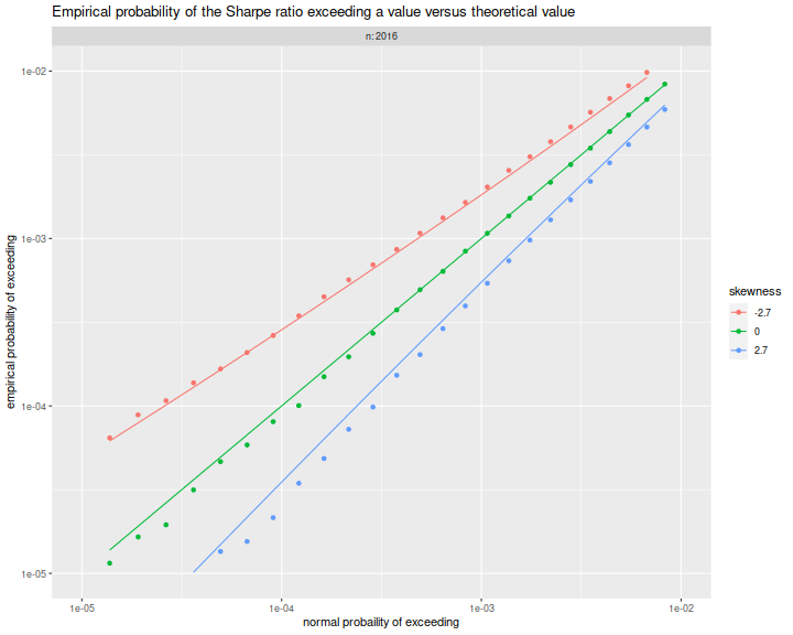
Here we plot the empirical exceedance probabilities versus $1 - \Phi\left(\frac{n}{n-1}\sqrt{n}q\right)$, with lines for the right hand side of the approximation above. We see that the approximation matches the experiments fairly well.

library(ggplot2)
ph <- resu %>%
  mutate(norm_law=pnorm(sqrt(n)*(n/(n-1))*vals,lower.tail=FALSE)) %>%
  mutate(hall_law=norm_law * exp(-(1/3)*((n*vals/(n-1))^3) * n * skewness)) %>%
  mutate(fskew=factor(signif(skewness,2))) %>%
  ggplot(aes(norm_law,prop,color=fskew,group=interaction(n,dl))) +
  geom_point() + 
  geom_line(aes(y=hall_law))+ 
  scale_x_log10(limits=c(1e-5,0.01)) + 
  scale_y_log10(limits=c(1e-5,0.01)) + 
  facet_wrap(~n,labeller=label_both) + 
  labs(x='normal probability of exceeding',
       y='empirical probability of exceeding',
       color='skewness',
       title='Empirical probability of the Sharpe ratio exceeding a value versus theoretical value')
print(ph)

A post-hoc test for the Sharpe ratio

Suppose you observe the historical returns of $p$ different fund managers, and wish to test whether any of them have superior Signal-Noise ratio (SNR) compared to the others. The first test you might perform is the test of pairwise equality of all SNRs. This test relies on the multivariate delta method and central limit theorem, resulting in a chi-square test, as described by Wright et al and outlined in section 4.3 of our Short Sharpe Course. This test is analogous to ANOVA, where one tests different populations for unequal means, assuming equal variance. (The equal Sharpe test, however, deals naturally with the case of paired observations, which is commonly the case in testing asset returns.)

In the analogous procedure, if one rejects the null of equal means in an ANOVA, one can perform pairwise tests for equality. This is called a post hoc test, since it is performed conditional on a rejection in the ANOVA. The basic post hoc test is Tukey's range test, sometimes called 'Honest Significant Differences'. It is natural to ask whether we can extend the same procedure to testing the SNR. Here we will propose such a procedure for a crude model of correlated returns.

The Tukey test has increased power by pooling all populations together to estimate the overall variance. The test statistic then becomes something like $$ \frac{Y_{(p)} - Y_{(1)}}{\sqrt{S^2 / n}}, $$ where $Y_{(1)}$ is the smallest mean observed, and $Y_{(p)}$ is the largest, and $S^2$ is the pooled estimate of variance. The difference between the maximal and minimal $Y$ is why this is called the 'range' test, since this is the range of the observed means.

Switching back to our problem, we should not have to assume that our tested returns series have the same volatility. Moreover, the standard error of the Sharpe ratio is only weakly dependent on the unknown population parameters, so we will not pool variances. In our paper on testing the asset with maximal Sharpe, we established that the vector of Sharpes, for normal returns and when the SNRs are small, is approximately asymptotically normal: $$ \hat{\zeta}\approx\mathcal{N}\left(\zeta,\frac{1}{n}R\right). $$ Here $R$ is the correlation of returns. See our previous blog post for more details. Under the null hypothesis that all SNRs are equal to $\zeta_0$, we can express this $$ z = \sqrt{n} \left(R^{1/2}\right)^{-1} \left(\hat{\zeta} - \zeta_0\right) \approx\mathcal{N}\left(0,I\right), $$ where $R^{1/2}$ is a matrix square root of $R$.

Now assume the simple rank-one model for correlation, where assets are correlated to a single common latent factor, but are otherwise independent: $$ R = \left(1-\rho\right) I + \rho 1 1^{\top}. $$ Under this model of $R$ we computed inverse-square-root of $R$ as $$ \left(R^{1/2}\right)^{-1} = \left(1-\rho\right)^{-1/2} I + \frac{1}{p}\left(\frac{1}{\sqrt{1-\rho+p\rho}} - \frac{1}{\sqrt{1-\rho}}\right)1 1^{\top}. $$

Picking two distinct indices, $i, j$ let $v = \left(e_i - e_j\right)$ be the contrast vector. We have $$ v^{\top}z = \frac{\sqrt{n}}{\sqrt{\left(1-\rho\right)}}v^{\top}\hat{\zeta}, $$ because $v^{\top}1=0$. Thus the range of the observed Sharpe ratios is a scalar multiple of the range of a set of $p$ independent standard normal variables. This is akin to the 'monotonicity' principle that we abused earlier when performing inference on the asset with maximum Sharpe.

Under normal approximation and the rank-one correlation model, we should then see $$ \left|\hat{\zeta}_{i} - \hat{\zeta}_{j}\right| \ge HSD = q_{1-\alpha,p,\infty} \sqrt{\frac{(1-\rho)}{n}}, $$ with probability $\alpha$, where the $q_{1-\alpha,m,n}$ is the upper $\alpha$-quantile of the Tukey distribution with $m$ and $n$ degrees of freedom. This is computed by qtukey in R. Alternatively one can construct confidence intervals around each $\hat{\zeta}_i$ of width $HSD$, whereby if another $\hat{\zeta}_j$ does not fall within it, the two are said to be Honestly Significantly Different. The familywise error rate should be no more than $\alpha$.

Testing

Let's test this under the null. We spawn 4 years of correlated returns from 16 managers, then compare the maximum and minimum observed Sharpe ratio, comparing them to the test value of $HSD$. Assume that the correlation is known to have value $\rho=0.8$. (More realistically, it would have to be estimated.) Note that for this many fund managers we have $$ q_{0.95,16,\infty}=4.85, $$ and thus taking into account the $\sqrt{1-\rho}$ term, $$ HSD = \frac{1}{\sqrt{n}} 2.17. $$ This is only slightly bigger than the naive approximate confidence intervals one would typically apply to the Sharpe ratio, which in this case would be around $$ \frac{\Phi^{-1}\left(0.975\right)}{\sqrt{n}} = \frac{1.96}{\sqrt{n}}. $$

We perform 10 thousand simulations, computing the Sharpe over all managers, and collecting the ranges. We compute the empirical type I error rate, and find it to be nearly equal to the nominal value of 0.05:

suppressMessages({
    library(mvtnorm)
})

nman <- 16
nyr  <- 4
ope  <- 252
SNR  <- 0.8   # annual units
rho  <- 0.8

nday <- round(nyr * ope)

R <- pmin(diag(nman) + rho,1)  
mu <- rep(SNR / sqrt(ope),nman)

nsim <- 10000
set.seed(1234)
ranges <- replicate(nsim,{
    X <- mvtnorm::rmvnorm(nday,mean=mu,sigma=R)
    zetahat <- colMeans(X) / apply(X,2,sd)
    max(zetahat) - min(zetahat)
})

alpha <- 0.05
HSDval <- sqrt((1-rho) / nday) * qtukey(alpha,lower.tail=FALSE,nmeans=nman,df=Inf)
mean(ranges > HSDval)

## [1] 0.0541

Compact Letter Display

The results of Tukey's test can be difficult to summarize. You might observe, for example, that managers 1 and 2 have significantly different SNRs, but not have enough evidence to say that 1 and 3 have different SNR, nor 2 and 3. How, then should you think about manager 3? He/She perhaps has the same SNR as 2, and perhaps the same as 1, but you have evidence that 1 and 2 have different SNR. You might label 1 as being among the 'high performers' and 2 among the 'average performers'; In which group should you place 3?

One answer would be to put manager 3 in both groups. This is a solution you might see as the result of compact letter displays, which is a commonly used way of communicating the results of multiple comparison procedures like Tukey's test. The idea is to put managers into multiple groups, each group identified by a letter, such that if two managers are in a common group, the HSD test fails to find they have significantly different SNR. The assignment to groups is actually not unique, and so subject to optimizing certain criteria, like minimizing the total number of groups, and so on, cf. Gramm et al. For our purposes here, we use Piepho's algorithm, which is conveniently provided by the multcompView package in R.

Here we apply the technique to the series of monthly returns of 5 industry factors, as compiled by Ken French, and published in his data library. We have almost 1200 months of data for these 5 returns. The returns are highly positively correlated, and we find that their common correlation is very close to 0.8. For this setup, and measuring the Sharpe in annualized units, the critical value at the 0.05 level is $$ HSD = \sqrt{12/n} 1.73. $$ For comparison, the half-width of the two sided confidence interval on the Sharpe in this case would be $$ \sqrt{12/n} 1.96, $$ which is a bit bigger. We have actually gained resolving power in our comparison of industries because of the high level of correlation.

Below we compute the observed Sharpe ratios of the five industries, finding them to range from around $0.49\,\mbox{year}^{-1/2}$ to $0.67\,\mbox{year}^{-1/2}$. We compute the HSD threshold, then call Piepho's method and print the compact letter display, shown below. In this case we require two groups, 'a' and 'b'. Based on our post hoc test, we assign Healthcare and Other into two different groups, but find no other honest significant differences, and so Consumer, Manufacturing and Technology get lumped into both groups.

# this is just a package of some data:
# if (!require(aqfb.data)) { install.packages('shabbychef/aqfb_data') }
library(aqfb.data)
data(mind5)

mysr <- colMeans(mind5) / apply(mind5,2,FUN=sd)
# sort decreasing for convenience later
mysr <- sort(mysr,decreasing=TRUE)
# annualize it
ope <- 12
mysr <- sqrt(ope) * mysr
# show
print(mysr)

##    Healthcare      Consumer Manufacturing    Technology         Other 
##        0.6674        0.6487        0.5967        0.5906        0.4852

srdiff <- outer(mysr,mysr,FUN='-')
R <- cov2cor(cov(mind5))
# this ends up being around 0.8:
myrho <- median(R[row(R) < col(R)])
alpha <- 0.05
HSD <- sqrt(ope) * sqrt((1-myrho) / nrow(mind5)) * qtukey(alpha,lower.tail=FALSE,nmeans=ncol(mind5),df=Inf)

library(multcompView)
lets <- multcompLetters(abs(srdiff) > HSD)
print(lets)

##    Healthcare      Consumer Manufacturing    Technology         Other 
##           "a"          "ab"          "ab"          "ab"           "b"

Distribution of Maximal Sharpe, Corrected Bonferroni

In a previous blog post we used the 'Polyhedral Inference' trick of Lee et al. to perform conditional inference on the asset with maximum Sharpe ratio. This is now a short paper on arxiv. I was somewhat disappointed to find, as noted in the paper, that polyhedral inference has lower power than a simple Bonferroni correction against alternatives where many assets have the same Signal-Noise ratio. (Though apparently it has higher power when one asset alone higher SNR.) The interpretation is that when there is no spread in the SNR, Bonferroni correction should have the same power as a single asset test, while conditional inference is sensitive to the conditioning information that you are testing a single asset which has Sharpe ratio perhaps near that of other assets. In the opposite case, Bonferroni suffers from having to 'pay' for a lot of irrelevant (for having low Sharpe) assets, while conditional inference does fine.

I also showed in the paper, as I demonstrated in a previous blog post, that the Bonferroni correction is conservative when asset returns are correlated. In a simple simulations under the null, I showed that the empirical type I rate goes to zero as common correlation $\rho$ goes to one. In this blog post I will describe a simple trick to correct for average positive correlation.

So let us suppose that we observe returns on $p$ assets over $n$ days, and that returns have correlation matrix $R$. Let $\hat{\zeta}$ be the vector of Sharpe ratios over this sample. In the paper I show that if returns are normal then the following approximation holds $$ \hat{\zeta}\approx\mathcal{N}\left(\zeta,\frac{1}{n}\left( R + \frac{1}{2}\operatorname{Diag}\left(\zeta\right)\left(R \odot R\right)\operatorname{Diag}\left(\zeta\right) \right)\right). $$ There is a more general form for Elliptically distributed returns. In the paper I find, via simulations, that for realistic SNRs and large sample sizes, the more general form does not add much accuracy. In fact, for the small SNRs one is likely to see in practice the simple approximation $$ \hat{\zeta}\approx\mathcal{N}\left(\zeta,\frac{1}{n}R\right) $$ will suffice.

Now note that, under the null hypothesis that $\zeta = \zeta_0$, one has $$ z = \sqrt{n} \left(R^{1/2}\right)^{-1} \left(\hat{\zeta} - \zeta_0\right) \approx\mathcal{N}\left(0,I\right), $$ where $R^{1/2}$ is a matrix square root of $R$. Testing the null hypothesis should proceed by computing (or estimating) the vector $z$, then comparing to normality, either by a Chi-square statistic, or performing Bonferroni-corrected normal inference on the largest element.

In the paper I used a simple rank-one model for correlation for simulations using $$ R = \left(1-\rho\right) I + \rho 1 1^{\top}. $$ This effectively models the influence of a common single 'latent' factor. Certainly this is more flexible for modeling real returns than assuming identity correlation, but is not terribly realistic.

Under this model of $R$ it is simple enough to compute the inverse-square-root of $R$. Namely $$ \left(R^{1/2}\right)^{-1} = \left(1-\rho\right)^{-1/2} I + \frac{1}{p}\left(\frac{1}{\sqrt{1-\rho+p\rho}} - \frac{1}{\sqrt{1-\rho}}\right)1 1^{\top}. $$ Let's just confirm with code:

p <- 4
rho <- 0.3
R <- (1-rho) * diag(p) + rho
ihR <- (1/sqrt(1-rho)) * diag(p) + (1/p) * ((1/sqrt(1-rho+p*rho)) - (1/sqrt(1-rho))) 
hR <- solve(ihR)
R - hR %*% hR

            [,1]        [,2]        [,3]        [,4]
[1,] 4.44089e-16 1.66533e-16 1.11022e-16 1.66533e-16
[2,] 1.66533e-16 0.00000e+00 5.55112e-17 5.55112e-17
[3,] 1.66533e-16 1.66533e-16 0.00000e+00 1.11022e-16
[4,] 1.11022e-16 1.11022e-16 1.11022e-16 2.22045e-16

So to test the null hypothesis, one computes $$ z = \sqrt{n} \left( \left(1-\rho\right)^{-1/2} I + \frac{1}{p}\left(\frac{1}{\sqrt{1-\rho+p\rho}} - \frac{1}{\sqrt{1-\rho}}\right)1 1^{\top} \right) \left(\hat{\zeta} - \zeta_0\right) $$ to test against normality. But note that our linear transformation is monotonic (indeed affine): if $v_i \ge v_j$ and $w = \left(R^{1/2}\right)^{-1} v$, then $w_i \ge w_j$. This means that the maximum element of $z$ has the same index as the maximum element of $\hat{\zeta} - \zeta_0$. To perform Bonferroni correction we need only transform the largest element of $\hat{\zeta} - \zeta_0$, by scaling it up, and shifting to accomodate the average. So if the largest element of $\hat{\zeta} - \zeta_0$ is $y$, and the average value is $a = \frac{1}{p}1^{\top} \left(\hat{\zeta} - \zeta_0\right)$, then the largest value of $z$ is $$ \frac{\sqrt{n} y}{\sqrt{1-\rho}} + a \sqrt{n} \left(\frac{1}{\sqrt{1-\rho+p\rho}} - \frac{1}{\sqrt{1-\rho}}\right) $$ Reject the null hypothesis if this is larger than $\Phi\left(1 - \alpha/p\right)$.

Simulations

Here we perform simple simulations of Bonferroni and corrected Bonferroni. We will assume that returns are Gaussian, that the correlation follows our simple rank one form, that the correlation is known in order to perform the corrected test. We simulate two years of daily data on 100 assets. For each choice of $\rho$ we perform 10000 simulations under the null of zero SNR, computing the simple and 'improved' Bonferroni corrected hypothesis tests. We tabulate the empirical type I rate and plot against $\rho$.

suppressMessages({
    library(dplyr)
    library(tidyr)
  library(future.apply)
})
# set up the functions
rawsim <- function(nday,nlatf,nsim=100,rho=0) {
  R <- pmin(diag(nlatf) + rho,1)  
  mu <- rep(0,nlatf)

    apart <- sqrt(nday)/sqrt(1-rho)
    bpart <- sqrt(nday) * ((1/sqrt(1-rho+nlatf*rho)) - (1/sqrt(1-rho)))

  mhtpvals <- replicate(nsim,{
        X <- mvtnorm::rmvnorm(nday,mean=mu,sigma=R)
        x <- colMeans(X) / apply(X,2,sd)
        bonf_pval <- nlatf * SharpeR::psr(max(x),df=nday-1,zeta=0,ope=1,lower.tail=FALSE) 
        # do the correction
        corr_stat <- apart * max(x) + bpart * mean(x)
        corr_pval <- nlatf * pnorm(corr_stat,lower.tail=FALSE)

    c(bonf_pval,corr_pval)
  })
  data_frame(bonf_pvals=as.numeric(mhtpvals[1,]),
                         corr_pvals=as.numeric(mhtpvals[2,]))
}
many_rawsim <- function(nday,nlatf,rho,nsim=1000L,nnodes=7) {
  if ((nsim > 10*nnodes) && require(future.apply)) {
        plan(multisession, workers = 7)  
        nper <- as.numeric(table(1:nsim %% nnodes))
    retv <- future_lapply(nper,function(aper) rawsim(nday=nday,nlatf=nlatf,rho=rho,nsim=aper)) %>%
      bind_rows()
        plan(sequential)
  } else {
        retv <- rawsim(nday=nday,nlatf=nlatf,rho=rho,nsim=nsim)
  }
  retv
}
mhtsim <- function(alpha=0.05,...) {
  many_rawsim(...) %>%
        tidyr::gather(key=method,value=pvalues) %>%
    group_by(method) %>%
      summarize(rej_rate=mean(pvalues < alpha)) %>%
    ungroup() %>%
    arrange(method)
}

# perform simulations
nsim <- 10000
nday <- 2*252
nlatf <- 100

params <- data_frame(rho=seq(0.01,0.99,length.out=7))

set.seed(123)
resu <- params %>%
  group_by(rho) %>%
    summarize(resu=list(mhtsim(nday=nday,nlatf=nlatf,rho=rho,nsim=nsim))) %>%
  ungroup() %>%
  unnest()

suppressMessages({
    library(dplyr)
    library(ggplot2)
})
# plot empirical rates:
ph <- resu %>%
    mutate(method=gsub('bonf_pvals','Plain Bonferroni',method)) %>%
    mutate(method=gsub('corr_pvals','Corrected Bonferroni',method)) %>%
  ggplot(aes(rho,rej_rate,color=method)) + 
  geom_line() + geom_point() + 
    geom_hline(yintercept=0.05,linetype=2,alpha=0.5) +
    scale_y_sqrt() + 
    labs(title='Empirical type I rate at the 0.05 level',
             x=expression(rho),y='type I rate',
             color='test')
print(ph)

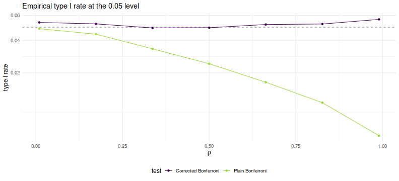
As desired, we maintain nominal coverage using the correction for $\rho$, while the naive Bonferroni is too conservative for large $\rho$. This is not yet a practical test, but could be used for rough estimation by plugging in the average sample correlation (or just SWAG'ing one). To my tastes a more interesting question is whether one can generalize this process to a rank $k$ approximation of $R$ while keeping the monotonicity property. (I have my doubts this is possible)