Distribution of Maximal Sharpe, Corrected Bonferroni
In a previous blog post we used the 'Polyhedral Inference' trick of Lee et al. to perform conditional inference on the asset with maximum Sharpe ratio. This is now a short paper on arxiv. I was somewhat disappointed to find, as noted in the paper, that polyhedral inference has lower power than a simple Bonferroni correction against alternatives where many assets have the same Signal-Noise ratio. (Though apparently it has higher power when one asset alone higher SNR.) The interpretation is that when there is no spread in the SNR, Bonferroni correction should have the same power as a single asset test, while conditional inference is sensitive to the conditioning information that you are testing a single asset which has Sharpe ratio perhaps near that of other assets. In the opposite case, Bonferroni suffers from having to 'pay' for a lot of irrelevant (for having low Sharpe) assets, while conditional inference does fine.
I also showed in the paper, as I demonstrated in a previous blog post, that the Bonferroni correction is conservative when asset returns are correlated. In a simple simulations under the null, I showed that the empirical type I rate goes to zero as common correlation $\rho$ goes to one. In this blog post I will describe a simple trick to correct for average positive correlation.
So let us suppose that we observe returns on $p$ assets over $n$ days, and that returns have correlation matrix $R$. Let $\hat{\zeta}$ be the vector of Sharpe ratios over this sample. In the paper I show that if returns are normal then the following approximation holds $$ \hat{\zeta}\approx\mathcal{N}\left(\zeta,\frac{1}{n}\left( R + \frac{1}{2}\operatorname{Diag}\left(\zeta\right)\left(R \odot R\right)\operatorname{Diag}\left(\zeta\right) \right)\right). $$ There is a more general form for Elliptically distributed returns. In the paper I find, via simulations, that for realistic SNRs and large sample sizes, the more general form does not add much accuracy. In fact, for the small SNRs one is likely to see in practice the simple approximation $$ \hat{\zeta}\approx\mathcal{N}\left(\zeta,\frac{1}{n}R\right) $$ will suffice.
Now note that, under the null hypothesis that $\zeta = \zeta_0$, one has $$ z = \sqrt{n} \left(R^{1/2}\right)^{-1} \left(\hat{\zeta} - \zeta_0\right) \approx\mathcal{N}\left(0,I\right), $$ where $R^{1/2}$ is a matrix square root of $R$. Testing the null hypothesis should proceed by computing (or estimating) the vector $z$, then comparing to normality, either by a Chi-square statistic, or performing Bonferroni-corrected normal inference on the largest element.
In the paper I used a simple rank-one model for correlation for simulations using $$ R = \left(1-\rho\right) I + \rho 1 1^{\top}. $$ This effectively models the influence of a common single 'latent' factor. Certainly this is more flexible for modeling real returns than assuming identity correlation, but is not terribly realistic.
Under this model of $R$ it is simple enough to compute the inverse-square-root of $R$. Namely $$ \left(R^{1/2}\right)^{-1} = \left(1-\rho\right)^{-1/2} I + \frac{1}{p}\left(\frac{1}{\sqrt{1-\rho+p\rho}} - \frac{1}{\sqrt{1-\rho}}\right)1 1^{\top}. $$ Let's just confirm with code:
p <- 4
rho <- 0.3
R <- (1-rho) * diag(p) + rho
ihR <- (1/sqrt(1-rho)) * diag(p) + (1/p) * ((1/sqrt(1-rho+p*rho)) - (1/sqrt(1-rho)))
hR <- solve(ihR)
R - hR %*% hR
            [,1]        [,2]        [,3]        [,4]
[1,] 4.44089e-16 1.66533e-16 1.11022e-16 1.66533e-16
[2,] 1.66533e-16 0.00000e+00 5.55112e-17 5.55112e-17
[3,] 1.66533e-16 1.66533e-16 0.00000e+00 1.11022e-16
[4,] 1.11022e-16 1.11022e-16 1.11022e-16 2.22045e-16
So to test the null hypothesis, one computes $$ z = \sqrt{n} \left( \left(1-\rho\right)^{-1/2} I + \frac{1}{p}\left(\frac{1}{\sqrt{1-\rho+p\rho}} - \frac{1}{\sqrt{1-\rho}}\right)1 1^{\top} \right) \left(\hat{\zeta} - \zeta_0\right) $$ to test against normality. But note that our linear transformation is monotonic (indeed affine): if $v_i \ge v_j$ and $w = \left(R^{1/2}\right)^{-1} v$, then $w_i \ge w_j$. This means that the maximum element of $z$ has the same index as the maximum element of $\hat{\zeta} - \zeta_0$. To perform Bonferroni correction we need only transform the largest element of $\hat{\zeta} - \zeta_0$, by scaling it up, and shifting to accomodate the average. So if the largest element of $\hat{\zeta} - \zeta_0$ is $y$, and the average value is $a = \frac{1}{p}1^{\top} \left(\hat{\zeta} - \zeta_0\right)$, then the largest value of $z$ is $$ \frac{\sqrt{n} y}{\sqrt{1-\rho}} + a \sqrt{n} \left(\frac{1}{\sqrt{1-\rho+p\rho}} - \frac{1}{\sqrt{1-\rho}}\right) $$ Reject the null hypothesis if this is larger than $\Phi\left(1 - \alpha/p\right)$.
Simulations
Here we perform simple simulations of Bonferroni and corrected Bonferroni. We will assume that returns are Gaussian, that the correlation follows our simple rank one form, that the correlation is known in order to perform the corrected test. We simulate two years of daily data on 100 assets. For each choice of $\rho$ we perform 10000 simulations under the null of zero SNR, computing the simple and 'improved' Bonferroni corrected hypothesis tests. We tabulate the empirical type I rate and plot against $\rho$.
suppressMessages({
    library(dplyr)
    library(tidyr)
  library(future.apply)
})
# set up the functions
rawsim <- function(nday,nlatf,nsim=100,rho=0) {
  R <- pmin(diag(nlatf) + rho,1)
  mu <- rep(0,nlatf)

    apart <- sqrt(nday)/sqrt(1-rho)
    bpart <- sqrt(nday) * ((1/sqrt(1-rho+nlatf*rho)) - (1/sqrt(1-rho)))

  mhtpvals <- replicate(nsim,{
        X <- mvtnorm::rmvnorm(nday,mean=mu,sigma=R)
        x <- colMeans(X) / apply(X,2,sd)
        bonf_pval <- nlatf * SharpeR::psr(max(x),df=nday-1,zeta=0,ope=1,lower.tail=FALSE)
        # do the correction
        corr_stat <- apart * max(x) + bpart * mean(x)
        corr_pval <- nlatf * pnorm(corr_stat,lower.tail=FALSE)

    c(bonf_pval,corr_pval)
  })
  data_frame(bonf_pvals=as.numeric(mhtpvals[1,]),
                         corr_pvals=as.numeric(mhtpvals[2,]))
}
many_rawsim <- function(nday,nlatf,rho,nsim=1000L,nnodes=7) {
  if ((nsim > 10*nnodes) && require(future.apply)) {
        plan(multisession, workers = 7)
        nper <- as.numeric(table(1:nsim %% nnodes))
    retv <- future_lapply(nper,function(aper) rawsim(nday=nday,nlatf=nlatf,rho=rho,nsim=aper)) %>%
      bind_rows()
        plan(sequential)
  } else {
        retv <- rawsim(nday=nday,nlatf=nlatf,rho=rho,nsim=nsim)
  }
  retv
}
mhtsim <- function(alpha=0.05,...) {
  many_rawsim(...) %>%
        tidyr::gather(key=method,value=pvalues) %>%
    group_by(method) %>%
      summarize(rej_rate=mean(pvalues < alpha)) %>%
    ungroup() %>%
    arrange(method)
}

# perform simulations
nsim <- 10000
nday <- 2*252
nlatf <- 100

params <- data_frame(rho=seq(0.01,0.99,length.out=7))

set.seed(123)
resu <- params %>%
  group_by(rho) %>%
    summarize(resu=list(mhtsim(nday=nday,nlatf=nlatf,rho=rho,nsim=nsim))) %>%
  ungroup() %>%
  unnest()
suppressMessages({
    library(dplyr)
    library(ggplot2)
})
# plot empirical rates:
ph <- resu %>%
    mutate(method=gsub('bonf_pvals','Plain Bonferroni',method)) %>%
    mutate(method=gsub('corr_pvals','Corrected Bonferroni',method)) %>%
  ggplot(aes(rho,rej_rate,color=method)) +
  geom_line() + geom_point() +
    geom_hline(yintercept=0.05,linetype=2,alpha=0.5) +
    scale_y_sqrt() +
    labs(title='Empirical type I rate at the 0.05 level',
             x=expression(rho),y='type I rate',
             color='test')
print(ph)
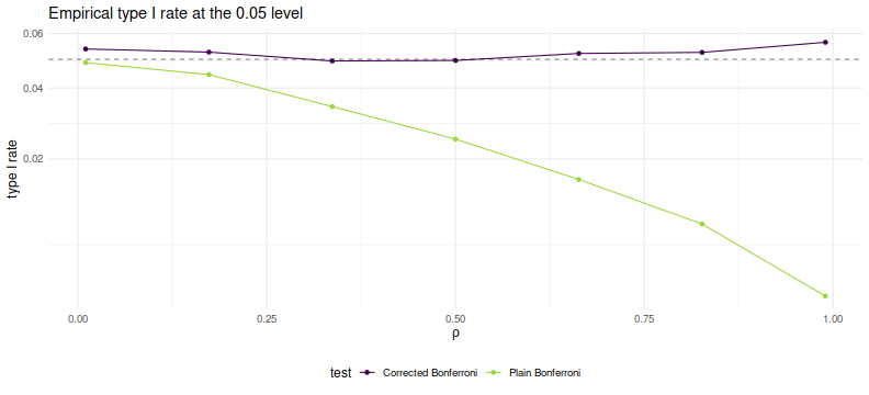
As desired, we maintain nominal coverage using the correction for $\rho$, while the naive Bonferroni is too conservative for large $\rho$. This is not yet a practical test, but could be used for rough estimation by plugging in the average sample correlation (or just SWAG'ing one). To my tastes a more interesting question is whether one can generalize this process to a rank $k$ approximation of $R$ while keeping the monotonicity property. (I have my doubts this is possible)