Distribution of Maximal Sharpe, Truncated Normal
In a previous blog post we looked at a symmetric confidence intervals on the Signal-Noise ratio. That study was motivated by the "opportunistic strategy", wherein one observes the historical returns of an asset to determine whether to hold it long or short. Then, conditional on the sign of the trade, we were able to construct proper confidence intervals on the Signal-Noise ratio of the opportunistic strategy's returns.
I had hoped that one could generalize from the single asset opportunistic strategy to the case of $p$ assets, where one constructs the Markowitz portfolio based on observed returns. I have not had much luck finding that generalization. However, we can generalize the opportunistic strategy in a different way to what I call the "Winner Take All" strategy. Here one observes the historical returns of $p$ different assets, then chooses the one with the highest observed Sharpe ratio to hold long. (Let us hold off on an Opportunistic Winner Take All.)
Observe, however, this is just the problem of inferring the Signal Noise ratio (SNR) of the asset with the maximal Sharpe. We previously approached that problem using a Markowitz approximation, finding it somewhat lacking. That Markowitz approximation was an attempt to correct some deficiencies with what is apparently the state of the art in the field, Marcos Lopez de Prado's (now AQR's?) "Most Important Plot in All of Finance", which is a thin layer of Multiple Hypothesis Testing correction over the usual distribution of the Sharpe ratio. In a previous blog post, we found that Lopez de Prado's method would have lower than nominal type I rates as it ignored correlation of assets.
Moreover, a simple MHT correction will not, I think, deal very well with the case where there are great differences in the Signal Noise ratios of the assets. The 'stinker' assets with low SNR will simply spoil our inference, unlikely to have much influence on which asset shows the highest Sharpe ratio, and only causing us to increase our significance threshold.
With my superior googling skills I recently discovered a 2013 paper by Lee et al, titled Exact Post-Selection Inference, with Application to the Lasso. While aimed at the Lasso, this paper includes a procedure that essentially solves our problem, giving hypothesis tests or confidence intervals with nominal coverage on the asset with maximal Sharpe among a set of possibly correlated assets.
The Lee et al paper assumes one observes $p$-vector $$ y \sim \mathcal{N}\left(\mu,\Sigma\right). $$ Then conditional on $y$ falling in some polyhedron, $Ay \le b$, we wish to perform inference on $\nu^{\top}y$. In our case the polyhedron will be the union of all polyhedra with the same maximal element of $y$ as we observed. That is, assume that we have reordered the elements of $y$ such that $y_1$ is the largest element. Then $A$ will be a column of negative ones, cbinded to the $p-1$ identity matrix, and $b$ will be a $p-1$ vector of zeros. The test is defined on $\nu=e_1$ the vector with a single one in the first element and zero otherwise.
Their method works by decomposing the condition $Ay \le b$ into a condition on $\nu^{\top}y$ and a condition on some $z$ which is normal but independent of $\nu^{\top}y$. You can think of this as kind of inverting the transform by $A$. After this transform, the value of $\nu^{\top}y$ is restricted to a line segment, so we need only perform inference on a truncated normal.
The code to implement this is fairly straightforward, and given below. The procedure to compute the quantile function, which we will need to compute confidence intervals, is a bit trickier, due to numerical issues. We give a hacky version below.
# Lee et. al eqn (5.8)
F_fnc <- function(x,a,b,mu=0,sigmasq=1) {
  sigma <- sqrt(sigmasq)
  phis <- pnorm((c(x,a,b)-mu)/sigma)
  (phis[1] - phis[2]) / (phis[3] - phis[2])
}
# Lee eqns (5.4), (5.5), (5.6)
Vfuncs <- function(z,A,b,ccc) {
  Az <- A %*% z
  Ac <- A %*% ccc
  bres <- b - Az
  brat <- bres
  brat[Ac!=0] <- brat[Ac!=0] / Ac[Ac!=0]
  Vminus <- max(brat[Ac < 0])
  Vplus  <- min(brat[Ac > 0])
  Vzero  <- min(bres[Ac == 0])
  list(Vminus=Vminus,Vplus=Vplus,Vzero=Vzero)
}
# Lee et. al eqn (5.9)
ptn <- function(y,A,b,nu,mu,Sigma,numu=as.numeric(t(nu) %*% mu)) {
  Signu <- Sigma %*% nu
  nuSnu <- as.numeric(t(nu) %*% Signu)
  ccc <- Signu / nuSnu  # eqn (5.3)
  nuy <- as.numeric(t(nu) %*% y)
  zzz <- y - ccc * nuy  # eqn (5.2)
  Vfs <- Vfuncs(zzz,A,b,ccc)
  F_fnc(x=nuy,a=Vfs$Vminus,b=Vfs$Vplus,mu=numu,sigmasq=nuSnu)
}
# invert the ptn function to find nu'mu at a given pval.
citn <- function(p,y,A,b,nu,Sigma) {
  Signu <- Sigma %*% nu
  nuSnu <- as.numeric(t(nu) %*% Signu)
  ccc <- Signu / nuSnu  # eqn (5.3)
  nuy <- as.numeric(t(nu) %*% y)
  zzz <- y - ccc * nuy  # eqn (5.2)
  Vfs <- Vfuncs(zzz,A,b,ccc)

  # you want this, but there are numerical issues:
  #f <- function(numu) { F_fnc(x=nuy,a=Vfs$Vminus,b=Vfs$Vplus,mu=numu,sigmasq=nuSnu) - p }
  sigma <- sqrt(nuSnu)
  f <- function(numu) {
    phis <- pnorm((c(nuy,Vfs$Vminus,Vfs$Vplus)-numu)/sigma)
    #(phis[1] - phis[2]) - p * (phis[3] - phis[2])
    phis[1] - (1-p) * phis[2] - p * phis[3]
  }
  # this fails sometimes, so find a better interval
  intvl <- c(-1,1)  # a hack.
  # this is very unfortunate
    trypnts <- seq(from=min(y),to=max(y),length.out=31)
    ys <- sapply(trypnts,f)
    dsy <- diff(sign(ys))
    if (any(dsy < 0)) {
      widx <- which(dsy < 0)
      intvl <- trypnts[widx + c(0,1)]
    } else {
      maby <- 2 * (0.1 + max(abs(y)))
      trypnts <- seq(from=-maby,to=maby,length.out=31)
      ys <- sapply(trypnts,f)
      dsy <- diff(sign(ys))
      if (any(dsy < 0)) {
        widx <- which(dsy < 0)
        intvl <- trypnts[widx + c(0,1)]
      }
    }
  uniroot(f=f,interval=intvl,extendInt='yes')$root
}
Testing on normal data
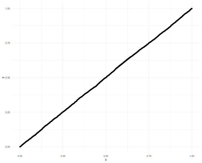
Here we test the code above on the problem considered in Theorem 5.2 of Lee et al. That is, we draw $y \sim \mathcal{N}\left(\mu,\Sigma\right)$, then observe the value of $F$ given in Theorem 5.2 when we plug in the actual population values of $\mu$ and $\Sigma$. This is several steps removed from our problem of inference on the SNR, but it is best to pause and make sure the implementation is correct first.
We perform 5000 simulations, letting $p=20$, then creating a random $\mu$ and $\Sigma$, drawing a single $y$, observing which element is the maximum, creating $A, b, \nu$, then computing the $F$ function, resulting in a $p$-value which should be uniform. We Q-Q plot those empirical $p$-values against a uniform law, finding them on the $y=x$ line.
gram <- function(x) { t(x) %*% x }
rWish <- function(n,p=n,Sigma=diag(p)) {
  require(mvtnorm)
  gram(rmvnorm(p,sigma=Sigma))
}
nsim <- 5000
p <- 20
A1 <- cbind(-1,diag(p-1))
set.seed(1234)
pvals <- replicate(nsim,{
  mu <- rnorm(p)
  Sigma <- rWish(n=2*p+5,p=p)
  y <- t(rmvnorm(1,mean=mu,sigma=Sigma) )
  # collect the maximum, so reorder the A above
  yord <- order(y,decreasing=TRUE)
  revo <- seq_len(p)
  revo[yord] <- revo

  A <- A1[,revo]
  nu <- rep(0,p)
  nu[yord[1]] <- 1
  b <- rep(0,p-1)
  foo <- ptn(y=y,A=A,b=b,nu=nu,mu=mu,Sigma=Sigma)
})
# plot them:
library(dplyr)
library(ggplot2)
ph <- data_frame(pvals=pvals) %>%
  ggplot(aes(sample=pvals)) +
  geom_qq(distribution=stats::qunif) +
  geom_qq_line(distribution=stats::qunif)
print(ph)
Now we attempt to use the confidence interval code. We construct a one-sided 95% confidence interval, and check how often it is violated by the $\mu$ of the element which shows the highest $y$. We will find that the empirical rate of violations of our confidence interval is indeed around 5%:
nsim <- 5000
p <- 20
A1 <- cbind(-1,diag(p-1))
set.seed(1234)
tgtval <- 0.95
viols <- replicate(nsim,{
  mu <- rnorm(p)
  Sigma <- rWish(n=2*p+5,p=p)
  y <- t(rmvnorm(1,mean=mu,sigma=Sigma) )
  # collect the maximum, so reorder the A above
  yord <- order(y,decreasing=TRUE)
  revo <- seq_len(p)
  revo[yord] <- revo

  A <- A1[,revo]
  nu <- rep(0,p)
  nu[yord[1]] <- 1
  b <- rep(0,p-1)
  # mu is unknown to this guy
  foo <- citn(p=tgtval,y=y,A=A,b=b,nu=nu,Sigma=Sigma)
  violated <- mu[yord[1]] < foo
})
print(sprintf('%.2f%%',100*mean(viols)))
[1] "5.04%"
Testing on the Sharpe ratio
To use this machinery to perform inference on the SNR, we can either port the results to the multivariate $t$-distribution, which seems unlikely because uncorrelated marginals of a multivariate $t$ are not independent. Instead we lean on the normal approximation to the vector of Sharpe ratios. If the $p$-vector $x$ is normal with correlation matrix $R$, then $$ \hat{\zeta}\approx\mathcal{N}\left(\zeta,\frac{1}{n}\left( R + \frac{1}{2}\operatorname{Diag}\left(\zeta\right)\left(R \odot R\right)\operatorname{Diag}\left(\zeta\right) \right)\right), $$ where $\hat{\zeta}$ is the $p$-vector of Sharpe ratios computed by observing $n$ independent draws of $x$, and $\zeta$ is the $p$-vector of Signal Noise ratios. Note how this generalizes the 'Lo' form of the standard error of a scalar Sharpe ratio, viz $\sqrt{(1 + \zeta^2/2)/n}$.
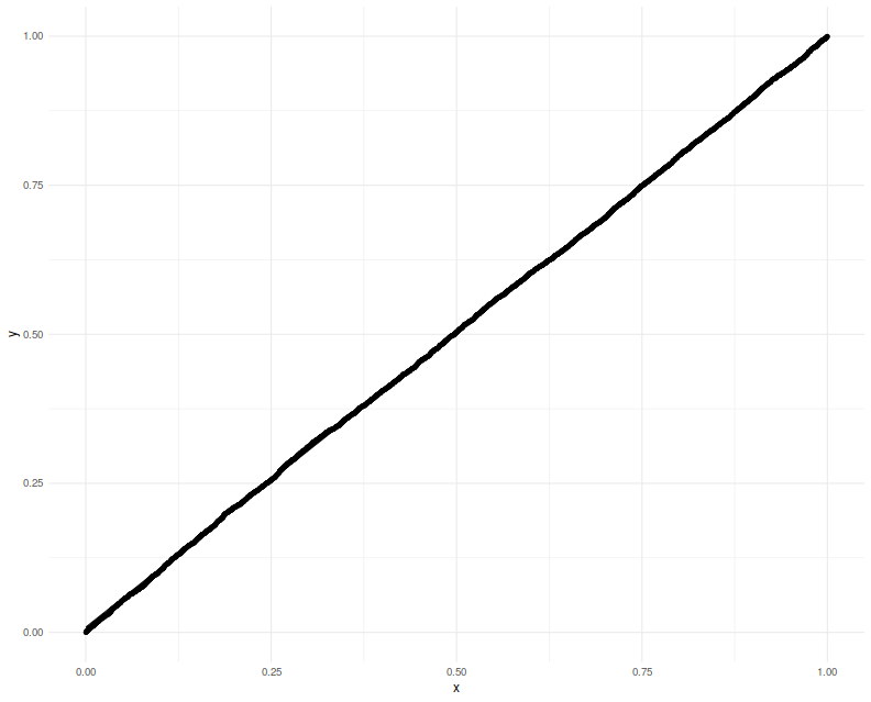
Here we will check the uniformity of $p$ values resulting from using this normal approximation. This is closer to the actual inference we want to do, except we will cheat by using the actual $R$ and $\zeta$ to construct what is essentially the $\Sigma$ to Lee's formulation. We will set $p=20$ and draw 3 years of daily data. Again we plot the putative $p$-values against uniformity and find a good match.
# let's test it!
nsim <- 5000
p <- 20
ndays <- 3 * 252
A1 <- cbind(-1,diag(p-1))
set.seed(4321)

pvals <- replicate(nsim,{
  # population values here
  mu <- rnorm(p)
  Sigma <- rWish(n=2*p+5,p=p)
  RRR <- cov2cor(Sigma)
  zeta <- mu /sqrt(diag(Sigma))

  Xrets <- rmvnorm(ndays,mean=mu,sigma=Sigma)
  srs <- colMeans(Xrets) / apply(Xrets,2,FUN=sd)

  y <- srs
  mymu <- zeta
  mySigma <- (1/ndays) * (RRR + (1/2) * diag(zeta) %*% (RRR * RRR) %*% diag(zeta))

  # collect the maximum, so reorder the A above
  yord <- order(y,decreasing=TRUE)
  revo <- seq_len(p)
  revo[yord] <- revo

  A <- A1[,revo]
  nu <- rep(0,p)
  nu[yord[1]] <- 1
  b <- rep(0,p-1)

  foo <- ptn(y=y,A=A,b=b,nu=nu,mu=mymu,Sigma=mySigma)
})
# plot them:
library(dplyr)
library(ggplot2)
ph <- data_frame(pvals=pvals) %>%
  ggplot(aes(sample=pvals)) +
  geom_qq(distribution=stats::qunif) +
  geom_qq_line(distribution=stats::qunif)
print(ph)
Lastly we make one more modification, filling in sample estimates for $\zeta$ and $R$ into the computation of the covariance. We compute one-sided 95% confidence intervals, and check how the empirical rate of violations. We find the rate to be around 5%.
nsim <- 5000
p <- 20
ndays <- 3 * 252
A1 <- cbind(-1,diag(p-1))
set.seed(9873)  # 5678 gives exactly 250 / 5000, which is eerie

tgtval <- 0.95
viols <- replicate(nsim,{
  # population values here
  mu <- rnorm(p)
  Sigma <- rWish(n=2*p+5,p=p)
  RRR <- cov2cor(Sigma)
  zeta <- mu /sqrt(diag(Sigma))

  Xrets <- rmvnorm(ndays,mean=mu,sigma=Sigma)
  srs <- colMeans(Xrets) / apply(Xrets,2,FUN=sd)
  Sighat <- cov(Xrets)
  Rhat <- cov2cor(Sighat)

  y <- srs
  # now use the sample approximations.
  # you can compute this from the observed information.
  mySigma <- (1/ndays) * (Rhat + (1/2) * diag(srs) %*% (Rhat * Rhat) %*% diag(srs))

  # collect the maximum, so reorder the A above
  yord <- order(y,decreasing=TRUE)
  revo <- seq_len(p)
  revo[yord] <- revo

  A <- A1[,revo]
  nu <- rep(0,p)
  nu[yord[1]] <- 1
  b <- rep(0,p-1)

  # mu is unknown to this guy
  foo <- citn(p=tgtval,y=y,A=A,b=b,nu=nu,Sigma=mySigma)
  violated <- zeta[yord[1]] < foo
})
print(sprintf('%.2f%%',100*mean(viols)))
[1] "5.14%"
Putting it together
Lee's method appears to give nominal coverage for hypothesis tests and confidence intervals on the SNR of the asset with maximal Sharpe. In principle it should not be affected by correlation of the assets or by large differences in the SNRs of the assets. It should be applicable in the $p > n$ case, as we are not inverting the covariance matrix. On the negative side, requiring one estimate the correlation of assets for the computation will not scale with large $p$.
We are guardedly optimistic that this method is not adversely affected by the normal approximation of the Sharpe ratio, although it would be ill-advised to use it for the case of small samples until more study is performed. Moreover the quantile function we hacked together here should be improved for stability and accuracy.