Distribution of Maximal Sharpe, the Markowitz Approximation

In a previous blog post we looked at a statistical test for overfitting of trading strategies proposed by Lopez de Prado, which essentially uses a $t$-test threshold on the maximal Sharpe of backtested returns based on assumed independence of the returns. (Actually it is not clear if Lopez de Prado suggests a $t$-test or relies on approximate normality of the $t$, but they are close enough.) In that blog post, we found that in the presence of mutual positive correlation of the strategies, the test would be somewhat conservative. It is hard to say just how conservative the test would be without making some assumptions about the situations in which it would be used.

This is a trivial point, but needs to be mentioned: to create a useful test of strategy overfitting, one should consider how strategies are developed and overfit. There are numerous ways that trading strategies are, or could be developed. I will enumerate some here, roughly in order of decreasing methodological purity:

Alice the Quant goes into the desert on a Vision Quest. She emerges three days later with a fully formed trading idea, and backtests it a single time to satisfy the investment committee. The strategy is traded unconditional on the results of that backtest.
Bob the Quant develops a black box that generates, on demand, a quantitative trading strategy, and performs a backtest on that strategy to produce an unbiased estimate of the historical performance of the strategy. All strategies are produced de novo, without any relation to any other strategy ever developed, and all have independent returns. The black box can be queried ad infinitum. (This is essentially Lopez de Prado's assumed mode of development.)
The same as above, but the strategies possibly have correlated returns, or were possibly seeded by published anomalies or trading ideas.
Carole the Quant produces a single new trading idea, in a white box, that is parametrized by a number of free parameters. The strategy is backtested on many settings of those parameters, which are chosen by some kind of design, and the settings which produce the maximal Sharpe are selected.
The same as above, except the parameters are optimized based on backtested Sharpe using some kind of hill-climbing heuristic or an optimizer.
The same as above, except the trading strategy was generally known and possibly overfit by other parties prior to publication as "an anomaly".
Doug the Quant develops a gray box trading idea, adding and removing parameters while backtesting the strategy and debugging the code, mixing machine and human heuristics, and leaving no record of the entire process.
A small group of Quants separately develop a bunch of trading strategies, using common data and tools, but otherwise independently hillclimb the in-sample Sharpe, adding and removing parameters, each backtesting countless unknown numbers of times, all in competition to have money allocated to their strategies.
The same, except the fund needs to have a 'good quarter', otherwise investors will pull their money, and they really mean it this time.

The first development mode is intentionally ludicrous. (In fact, these modes are also roughly ordered by increasing realism.) It is the only development model that might result in underfitting. The division between the second and third modes is loosely quantifiable by the mutual correlation among strategies, as considered in the previous blog post. But it is not at all clear how to approach the remaining development modes with the maximal Sharpe statistic. Perhaps a "number of pseudo-independent backtests" could be estimated and then used with the proposed test, but one cannot say how this would work with in-sample optimization, or the diversification benefit of looking in multidimensional parameter space.

The Markowitz Approximation

Perhaps the maximal Sharpe test can be salvaged, but I come to bury Caesar, not to resuscitate him. Some years ago, I developed a test for overfitting based on an approximate portfolio problem. I am ashamed to say, however, that while writing this blog post I have discovered that this approximation is not as accurate as I had remembered! It is interesting enough to present, I think, warts and all.

Suppose you could observe the time series of backtested returns from all the backtests considered. By 'all', I want to be very inclusive if the parameters were somehow optimized by some closed form equation, say. Let $Y$ be the $n \times k$ matrix of returns, with each row a date, and each column one of the backtests. We suppose we have selected the strategy which maximizes Sharpe, which corresponds to picking the column of $Y$ with the largest Sharpe.

Now perform some kind of dimensionality reduction on the matrix $Y$ to arrive at

$$ Y \approx X W, $$

where $X$ is an $n \times l$ matrix, and $W$ is an $l \times k$ matrix, and where $l \ll k$. The columns of $X$ approximately span the columns of $Y$. Picking the strategy with maximal Sharpe now approximately corresponds to picking a column of $W$ that has the highest Sharpe when multiplied by $X$. That is, our original overfitting approximately corresponded to the optimization problem

$$ \max_{w \in W} \operatorname{Sharpe}\left(X w\right). $$

The unconstrained version of this optimization problem is solved by the Markowitz portfolio. Moreover, if the returns $X$ are multivariate normal with independent rows, then the distribution of the (squared) Sharpe of the Markowitz portfolio is known, both under the null hypothesis (columns of $X$ are all zero mean), and the alternative (the maximal achievable population Sharpe is non-zero), via Hotelling's $T^2$ statistic.

If $\hat{\zeta}$ is the (in-sample) Sharpe of the (in-sample) Markowitz portfolio on $X$, assumed i.i.d. Normal, then

$$ \frac{(n-l) \hat{\zeta}^2}{l (n - 1)} $$

follows an F distribution with $l$ and $n-l$ degrees of freedom. I wrote the psropt and qsropt functions in SharpeR to compute the CDF and quantile of the maximal in-sample Sharpe to support this kind of analysis.

I should note there are a few problems with this approximation:

There is no strong theoretical basis for this approximation: we do not have a model for how correlated returns should arise for a particular population, nor what the dimension $l$ should be, nor what to expect under the alternative, when the true optimal strategy has positive Sharpe. (I suspect that posing overfit of backtests as a Gaussian Process might be fruitful.)
We have to estimate the dimensionality, $l$, which is about as odious as estimating the number of 'pseudo-observations' in the maximal Sharpe test. I had originally suspected that $l$ would be 'obvious' from the application, but this is not apparently so.
Although the returns may live nearly in an $l$ dimensional subspace, we might have have selected a suboptimal combination of them in our overfitting process. This would be of no consequence if the $l$ were accurately estimated, but it will stymie our testing of the approximation.

Despite these problems, let us press on.

An example: a two window Moving Average Crossover

While writing this blog post, I went looking for examples of 'classical' technical strategies which would be ripe for overfitting (and which I could easily simulate under the null hypothesis). I was surprised to find that freely available material on Technical Analysis was even worse than I could imagine. Nowhere among the annotated plots with silly drawings could I find a concrete description of a trading strategy, possibly with free parameters to be fit to the data. Rather than wade through that swamp any longer, I went with an old classic, the Moving Average Crossover.

The idea is simple: compute two moving averages of the price series with different windows. When one is greater than the other, hold the asset long, otherwise hold it short. The choice of two windows must be overfit by the quant. Here I perform that experiment, but under the null hypothesis, with zero mean simulated returns generated independently of each other. Any realization of this strategy, with any choice of the windows, will have zero mean returns and thus zero Sharpe.

First I collect 'backtests' (sans any trading costs) of two window MAC for a single realization of returns where the two windows were allowed to vary from 2 to around 1000. The backtest period is 5 years of daily data. I compute the singular value decomposition of the returns, then present a scree plot of the singular values.

suppressMessages({
  library(dplyr)
  library(fromo)
    library(svdvis)
})
# return time series of *all* backtests
backtests <- function(windows,rel_rets) {
    nwin <- length(windows)
    nc <- choose(nwin,2) 

    fwd_rets <- dplyr::lead(rel_rets,1)
    # log returns
    log_rets <- log(1 + rel_rets)
    # price series
    psers <- exp(cumsum(log_rets))
    avgs <- lapply(windows,fromo::running_mean,v=psers)

    X <- matrix(0,nrow=length(rel_rets),ncol=2*nc)

    idx <- 1
    for (iii in 1:(nwin-1)) {
        for (jjj in (iii+1):nwin) {
            position <- sign(avgs[[iii]] - avgs[[jjj]])
            myrets <- position * fwd_rets
            X[,idx] <- myrets
            X[,idx+1] <- -myrets
            idx <- idx + 1
        }
    }
    # trim the last row, which has the last NA
    X <- X[-nrow(X),]
    X
}
geomseq <- function(from=1,to=1,by=(to/from)^(1/(length.out-1)),length.out=NULL) {
    if (missing(length.out)) { 
        lseq <- seq(log(from),log(to),by=log(by)) 
    } else {
        lseq <- seq(log(from),log(to),by=log(by),length.out=length.out)
    }
    exp(lseq)
}

# which windows to test
windows <- unique(ceiling(geomseq(2,1000,by=1.15))) 
nobs <- ceiling(3 * 252)
maxwin <- max(windows)
rel_rets <- rnorm(maxwin + 10 + nobs,mean=0,sd=0.01)

XX <- backtests(windows,rel_rets)
# grab the last nobs rows
XX <- XX[(nrow(XX)-nobs+1):(nrow(XX)),]

# perform svd
blah <- svd(x=XX,nu=11,nv=11)
# look at it
ph <- svdvis::svd.scree(blah) +
    labs(x='Singular Vectors',y='Percent Variance Explained') 
print(ph)

plot of chunk mac_one_sim_scree

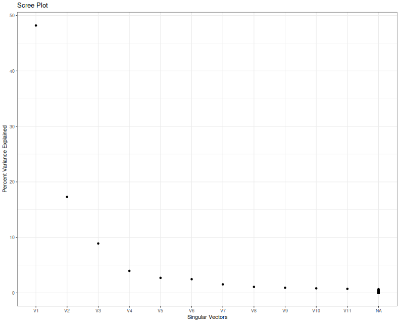
I think we can agree that nobody knows how to interpret a scree plot. However, in this case a large proportion of the explained variance seems to encoded in the first two eigenvalues, which is consistent with my a priori guess that $l=2$ in this case because of the two free parameters.

Next I simulate overfitting, performing that same experiment, but picking the largest in-sample Sharpe ratio. I create a series of independent zero mean returns, then backtest a bunch of MAC strategies, and save the maximal Sharpe over a 3 year window of daily data. I repeat this experiment ten thousand times, and then look at the distribution of that maximal Sharpe.

suppressMessages({
  library(dplyr)
  library(tidyr)
  library(tibble)
  library(SharpeR)
  library(future.apply)
  library(ggplot2)
})
ope <- 252

geomseq <- function(from=1,to=1,by=(to/from)^(1/(length.out-1)),length.out=NULL) {
    if (missing(length.out)) { 
        lseq <- seq(log(from),log(to),by=log(by)) 
    } else {
        lseq <- seq(log(from),log(to),by=log(by),length.out=length.out)
    }
    exp(lseq)
}
# one simulation. returns maximal Sharpe
onesim <- function(windows,n=1000) {
    maxwin <- max(windows)
    rel_rets <- rnorm(maxwin + 10 + n,mean=0,sd=0.01)
    fwd_rets <- dplyr::lead(rel_rets,1)
    # log returns
    log_rets <- log(1 + rel_rets)
    # price series
    psers <- exp(cumsum(log_rets))
    avgs <- lapply(windows,fromo::running_mean,v=psers)

    nwin <- length(windows)
    maxsr <- 0

    for (iii in 1:(nwin-1)) {
        for (jjj in (iii+1):nwin) {
            position <- sign(avgs[[iii]] - avgs[[jjj]])
            myrets <- position * fwd_rets
            # compute Sharpe on some part of this
            compon <- myrets[(length(myrets)-n):(length(myrets)-1)]
            thissr <- SharpeR::as.sr(compon,ope=ope)$sr
            # we are implicitly testing both combinations of long and short here,
            # so we take the absolute Sharpe, since we will always overfit to
            # the better of the two:
            maxsr <- max(maxsr,abs(thissr))
        }
    }
    maxsr
}

windows <- unique(ceiling(geomseq(2,1000,by=1.15))) 
nobs <- ceiling(3 * 252)
nrep <- 10000
plan(multiprocess)
set.seed(1234)
system.time({
    simvals <- future_replicate(nrep,onesim(windows,n=nobs))
})

    user   system  elapsed 
1522.724    5.978  271.297

Here I plot the empirical quantiles of the maximal (annualized) Sharpe versus theoretical quantiles under the Markowitz approximation, assuming $l=2$. I also plot the $y=x$ lines, and horizontal and vertical lines at the nominal upper $0.05$ cutoff based on the Markowitz approximation.

# plot max value vs quantile
library(ggplot2)
apxdf <- 2.0
ph <- data.frame(simvals=simvals) %>%
    ggplot(aes(sample=simvals)) + 
    geom_vline(xintercept=SharpeR::qsropt(0.95,df1=apxdf,df2=nobs,zeta.s=0,ope=ope),linetype=3) +
    geom_hline(yintercept=SharpeR::qsropt(0.95,df1=apxdf,df2=nobs,zeta.s=0,ope=ope),linetype=3) +
    stat_qq(distribution=SharpeR::qsropt,dparams=list(df1=apxdf,df2=nobs,zeta.s=0,ope=ope)) +
    geom_abline(intercept=0,slope=1,linetype=2) + 
    labs(title='empirical quantiles of maximal Sharpe versus Markowitz Approximation',
             x='theoretical quantile',y='empirical quantile (Sharpe in annual units)')
print(ph)

plot of chunk mac_sims_qq

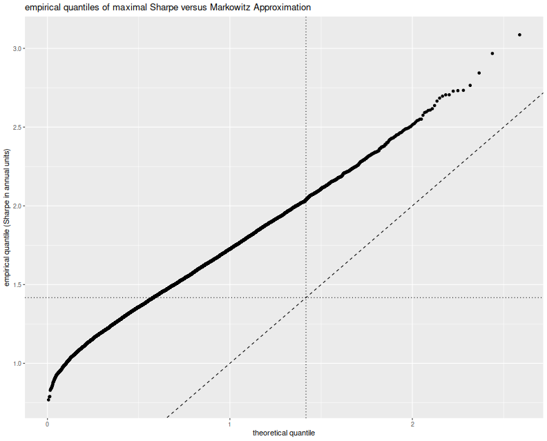
This approximation is clearly no good. The empirical rate of type I errors at the $0.05$ level is around 60%, and the Q-Q line is just off. I must admit that when I previously looked at this approximation (and in the vignette for SharpeR!) I used the qqline function in base R, which fits a line based on the first and third quartile of the empirical fit. That corresponds to an affine shift of the line we see here, and nothing seems amiss.

So perhaps the Markowitz approximation can be salvaged, if I can figure out why this shift occurs. Perhaps we have only traded picking a maximal $t$ for picking a maximal $T^2$ and there still has to be a mechanism to account for that. Or perhaps in this case, despite the 'obvious' setting of $l=2$, we should have chosen $l=7$, for which the empirical rate of type I errors is around 60%, though we have no way of seeing that 7 from the scree plot or by looking at the mechanism for generating strategies. Or perhaps the problem is that we have not actually picked a maximal strategy over the subspace, and this technique can only be used to provide a possibly conservative test. In this regard, our test would be no more useful than the maximal Sharpe test described in the previous blog post.

posted at 09:09 · blog · sharpe-ratio quant-finance analysis statistics max-sharpe Markowitz R

Sharpe Ratio

Jul 14, 2018