I recently ran across what Marcos Lopez de Prado calls
"The most important plot in Finance".
As I am naturally antipathetic to such outsized, self-aggrandizing
claims I was resistant to drawing attention to it.
However, what it purports to correct is a serious problem
in quantitative trading, namely backtest overfit (variously known
elsewhere as data-dredging, p-hacking, etc.).
Suppose you had some process that would, on demand, generate a trading
strategy, backtest it, and present you (somehow) with an unbiased estimate
of the historical performance of that strategy. This process might be
random generation a la genetic programming, some other automated process,
or a small army of very eager quants ("grad student descent"). If you had
access to such a process, surely you would query it hundreds or even
thousands of times, much like a slot machine, to get the best strategy.
Before throwing money at the best strategy, first you have
to identify it (probably via the Sharpe ratio on the backtested returns,
or some other heuristic objective), then you should probably assess whether
it is any good, or simply the result of "dumb luck". More formally, you
might perform a hypothesis test under the null hypothesis that all the
generated strategies have non-positive expected returns, or you might
try to construct a confidence interval on the Signal-Noise ratio of
the strategy with best in-sample Sharpe.
The "Most Important Plot" in all finance is, apparently, a representation
of the distribution of the maximal in-sample Sharpe ratio of $B$ different
backtests over strategies that are zero mean, and have independent returns,
versus that $B$. As presented by its author it is a heatmap, though
I imagine boxplots or violin plots would be easier to digest. To generate
this plot, note that the smallest value of $B$ independent uniform random
variates takes a Beta distribution
with parameters $1$ and $B$. So to find the $q$th quantile of the maximum
Sharpe, compute the $1-q$ quantile of the $\beta\left(1,B\right)$ distribution,
then plug that the quantile function of the Sharpe distribution with the right
degrees of freedom and zero Signal Noise parameter. (See Exercise 3.29 in my
Short Sharpe Course.)
In theory this should give you a significance threshold against which you can
compare your observed maximal Sharpe. If yours is higher, presumably you should
trade the strategy (uhh, after you pay Marcos for using his patented
technology), otherwise give up quantitative trading and become an accountant.
One huge problem with this Most Important Plot method (besides its ignorance of
entire fields of research on Multiple Hypothesis Testing, False
Discovery Rate, Estimation After Selection, White's Reality Check, Romano-Wolf,
Politis, Hansen's SPA, inter alia) is the assumption of independence.
"Assuming quantities are independent which are not independent" is the downfall
of many a statistical procedure applied in the wild (much more so than
non-normality), and here is no different.
And we have plenty of reason to believe returns from any real strategy
generation process would fail independence:
- Strategies are typically generated on a limited universe of assets,
and using a limited set of predictive 'features', and are tested
on a single, often relatively short, history.
- Most strategy generation processes (synthetic and human) have a very
limited imagination.
- Most strategy generation processes (synthetic and human) tend to work
incrementally, generating new strategies
after having observed the in-sample performance of existing strategies.
They "hill-climb".
My initial intuition was that dependence among strategies, especially of the
hill-climbing variety, would cause this Most Important Test to have a much
higher rate of type I errors than advertised. (This would be bad, since it
would effectively still pass dud trading strategies while selling you a
false sense of security.) However, it seems that the more innocuous correlation
of random generation on a limited set of strategies and assets causes
this test to be conservative. (It is similar to Bonferroni's correction in this
regard.)
To establish this conservatism, you can
use Slepian's Lemma. This
lemma is a kind of stochastic dominance result for multivariate normals.
It says that if $X$ and $Y$ are $B$-variate normal random variables,
where each element is zero mean and unit variance, and if the covariance
of any pair of elements of $X$ is no less than the covariance of the
corresponding pair of elements of $Y$, then $Y$ stochastically dominates
$X$, in the multivariate sense. This is actually a stronger result than
what we need, which is stochastic dominance of the maximal element of $Y$
over the maximal element of $X$, which it implies.
Here I simply illustrate this dominance empirically. I create a $B$-variate
normal with zero mean and unit variance of marginals, for $B=1000$.
The elements are all correlated to each other with correlation $\rho$.
I compute the maximum over the $B$ elements. I perform this simulation
100 thousand times, then compute the $q$th empirical quantile over the
$10^5$ maximum values. I vary $\rho$ from 0 to 0.75. Here is the code:
suppressMessages({
  library(dplyr)
  library(tidyr)
  library(tibble)
  library(broom)
  library(ggplot2)
  library(future.apply)
})
# one (bunch of) simulation.
onesim <- function(B,rho=0,propcor=1.0,nsims=100L) {
    propcor <- min(1.0,max(propcor,1-propcor))
    rho <- abs(rho)
    # (anti)correlated part; each row is a simulation
    X0 <- outer(array(rnorm(nsims)),array(2*rbinom(B,size=1,prob=propcor)-1))
    # idiosyncratic part
    XF <- matrix(rnorm(B*nsims),nrow=nsims,ncol=B)
    XX <- sqrt(rho) * X0 + sqrt(1-rho) * XF
    data_frame(maxval=apply(XX,1,FUN="max"))
}
# many sims.
repsim <- function(B,rho=0,propcor=1.0,nsims=1000L) {
    maxper <- 100L
    nreps <- ceiling(nsims / maxper)
  jumble <- replicate(nreps,onesim(B=B,rho=rho,propcor=propcor,nsims=maxper),simplify=FALSE) %>%
        bind_rows()
}
manysim <- function(B,rho=0,propcor=1.0,nsims=10000L,nnodes=7) {
  if ((nsims > 100*nnodes) && require(future.apply)) {
        plan(multisession, workers = 7)
    # do in parallel.
        nper <- ceiling(nsims / nnodes)
    retv <- future_lapply(1:nnodes, function(ignore) repsim(B=B,rho=rho,propcor=propcor,nsims=nper)) %>%
      bind_rows()
        plan(sequential)
        retv <- retv[1:nsims,]
  } else {
        retv <- repsim(B=B,rho=rho,propcor=propcor,nsims=nsims)
  }
  retv
}

params <- tidyr::crossing(data_frame(rho=c(0,0.25,0.5,0.75)),
                                                    data_frame(propcor=c(0.5,1.0))) %>%
  dplyr::filter(rho > 0 | propcor == 1)

# run a bunch;
nrep <- 1e5
set.seed(1234)
system.time({
    results <- params %>%
        group_by(rho,propcor) %>%
            summarize(sims=list(manysim(B=1000,rho=rho,propcor=propcor,nsims=nrep))) %>%
        ungroup() %>%
        tidyr::unnest(cols=c(sims))
})
   user  system elapsed
  3.522   0.314  44.945
# aggregate the results
do_aggregate <- function(results) {
    results %>%
        group_by(rho,propcor) %>%
            summarize(qs=list(broom::tidy(quantile(maxval,probs=seq(0.50,0.9975,by=0.0025))))) %>%
        ungroup() %>%
        tidyr::unnest(cols=c(qs)) %>%
        rename(qtile=names,value=x)
}
sumres <- results %>% do_aggregate()
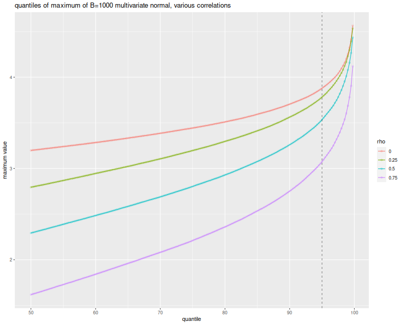
Here I plot the empirical $q$th quantile of the maximum versus $q$, with
different lines for the different values of $\rho$. I include a vertical
line at the 0.95 quantile, to show where the nominal 0.05 level threshold is.
The takeaway, as implied by Slepian's lemma, is that the maximum over $B$ Gaussian elements decreases
stochastically as the correlation of elements increases.
Thus when you assume independence of your backtests, you use the red line as your
significance threshold (typically where it intersects the dashed vertical line),
while your processes live on the green or blue or purple lines. Your test will
be too conservative, and your true type I rate will be lower than the nominal
rate.
# plot max value vs quantile
library(ggplot2)
ph <- sumres %>%
    dplyr::filter(propcor==1) %>%
    mutate(rho=factor(rho)) %>%
    mutate(xv=as.numeric(gsub('%$','',qtile))) %>%
    ggplot(aes(x=xv,y=value,color=rho,group=rho)) +
    geom_line() + geom_point(alpha=0.2) +
    geom_vline(xintercept=95,linetype=2,alpha=0.5) +    # the 0.05 significance cutoff
    labs(title='quantiles of maximum of B=1000 multivariate normal, various correlations',
             x='quantile',y='maximum value')
print(ph)
But wait, these simulations were over Gaussian vectors (and Slepian's Lemma is only
applicable in the Gaussian case), while the
Most Important Test is to be applied to the Sharpe ratio. They have different distributions.
It turns out, however, that when the population mean is the zero vector, the vector of Sharpe ratios
of returns with correlation matrix $R$ is approximately normal with
variance-covariance matrix $\frac{1}{n} R$. (This is in section 4.2 of
Short Sharpe Course.)
Here I establish that empirically, by performing the same simulations again,
this time spawning 252 days of normally distributed returns with zero mean, for
$B$ possibly correlated strategies, computing their Sharpes, and taking the
maximum. I only perform $10^4$ simulations because this one is quite a bit
slower:
# really just one simulation.
onesim <- function(B,nday,rho=0,propcor=1.0,pzeta=0) {
    propcor <- min(1.0,max(propcor,1-propcor))
    rho <- abs(rho)
    # correlated part; each row is one day
    X0 <- outer(array(rnorm(nday)),array(2*rbinom(B,size=1,prob=propcor)-1))
    # idiosyncratic part
    XF <- matrix(rnorm(B*nday),nrow=nday,ncol=B)
    XX <- pzeta + (sqrt(rho) * X0 + sqrt(1-rho) * XF)
    sr <- colMeans(XX) / apply(XX,2,FUN="sd")
    # if you wanted to look at them cumulatively:
    #data_frame(maxval=cummax(sr),iterate=1:B)
    # otherwise just the maxval
    data_frame(maxval=max(sr),iterate=B)
}
# many sims.
repsim <- function(B,nday,rho=0,propcor=1.0,pzeta=0,nsims=1000L) {
  jumble <- replicate(nsims,onesim(B=B,nday=nday,rho=rho,propcor=propcor,pzeta=pzeta),simplify=FALSE) %>%
        bind_rows()
}
manysim <- function(B,nday,rho=0,propcor=1.0,pzeta=0,nsims=1000L,nnodes=7) {
  if ((nsims > 10*nnodes) && require(future.apply)) {
        plan(multisession, workers = 7)
    # do in parallel.
        nper <- as.numeric(table(1:nsims %% nnodes))
    retv <- future_lapply(nper, function(aper)
      repsim(B=B,nday=nday,rho=rho,propcor=propcor,pzeta=pzeta,nsims=aper)) %>%
      bind_rows()
        plan(sequential)
  } else {
        retv <- repsim(B=B,nday=nday,rho=rho,propcor=propcor,pzeta=pzeta,nsims=nsims)
  }
  retv
}

params <- tidyr::crossing(data_frame(rho=c(0,0.25,0.5,0.75)),
                                                    data_frame(propcor=c(1.0))) %>%
  dplyr::filter(rho > 0 | propcor == 1)

# run a bunch;
nday <- 252
numbt <- 1000
nrep <- 1e4
# should take around 8 minutes on 7 cores
set.seed(1234)
system.time({
    sh_results <- params %>%
        group_by(rho,propcor) %>%
            summarize(sims=list(manysim(B=numbt,nday=nday,propcor=propcor,pzeta=0,rho=rho,nsims=nrep))) %>%
        ungroup() %>%
        tidyr::unnest(cols=c(sims))
})
   user  system elapsed
 22.499   0.889 548.267
# aggregate
sh_sumres <- sh_results %>%
    dplyr::filter(iterate==1000) %>%
    do_aggregate() %>%
    mutate(value=sqrt(252) * value)   # annualize!
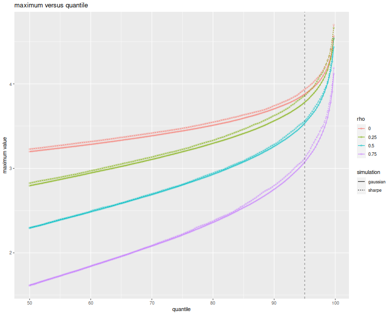
Again, I plot the empirical $q$th quantile of the maximum Sharpe, in annualized units,
versus $q$, with different lines for the different values of $\rho$. Because
we take one year of returns and annualize the Sharpe, the test statistics
should be approximately normal with approximately unit marginal variances. This
plot should look eerily similar to the one above, so I overlay the Sharpe
simulation results with the results of the Gaussian experiment above to show
how close they are. Very little has been lost in the normal approximation to
the sample Sharpe, but the maximal Sharpes are slightly elevated compared
to the Gaussian case.
# plot max value vs quantile
library(ggplot2)
ph <- sh_sumres %>%
    mutate(simulation='sharpe') %>%
    rbind(sumres %>% mutate(simulation='gaussian')) %>%
    dplyr::filter(propcor==1) %>%
    mutate(rho=factor(rho)) %>%
    mutate(xv=as.numeric(gsub('%$','',qtile))) %>%
    ggplot(aes(x=xv,y=value,color=rho,linetype=simulation)) +
    geom_line() + geom_point(alpha=0.2) +
    geom_vline(xintercept=95,linetype=2,alpha=0.5) +    # the 0.05 significance cutoff
    labs(title='maximum versus quantile',x='quantile',y='maximum value')
print(ph)
The simulations here show what can happen when many strategies have mutual positive correlation.
One might wonder what would happen if there were many strategies with a
significant negative correlation. It turns out this is not really possible.
In order for the correlation matrix to be positive definite, you cannot have
too many strongly negative off-diagonal elements. Perhaps there is a Pigeonhole
Principle argument for this, but a
simple expectation argument suffices.
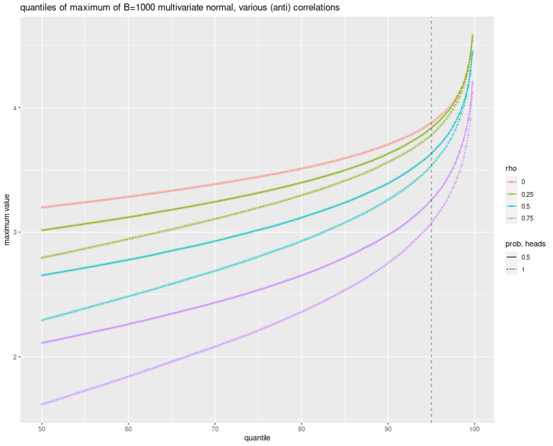
Just in case, however, above I also simulated the case where you flip a coin to
determine whether an element of the Gaussian has a positive or negative
correlation to the common element. When the coin is completely biased to heads,
you get the simulations shown above. When the coin is fair, the elements of the
Gaussian are expected to be divided evenly into two highly groups. Here is the
plot of the $q$th quantile of the maximum versus $q$, with different colors for
$\rho$ and different lines for the probability of heads. Allowing
negatively correlated elements does stochastically increase the maximum
element, but never above the $\rho=0$ case. And so the Most Important Test
still appears conservative.
# plot max value vs quantile:
library(ggplot2)
ph <- sumres %>%
    mutate(rho=factor(rho)) %>%
    mutate(`prob. heads`=factor(propcor)) %>%
    mutate(xv=as.numeric(gsub('%$','',qtile))) %>%
    ggplot(aes(x=xv,y=value,color=rho,linetype=`prob. heads`)) +
    geom_line() + geom_point(alpha=0.2) +
    geom_vline(xintercept=95,linetype=2,alpha=0.5) +    # the 0.05 significance cutoff
    labs(title='quantiles of maximum of B=1000 multivariate normal, various (anti) correlations',
             x='quantile',y='maximum value')
print(ph)
In a followup post I will attempt to address the conservatism and hill-climbing
issues, using the Markowitz approximation.
Click to read and post comments
That the Sharpe ratio is biased is not unknown;
this was established for Gaussian returns by Miller and Gehr in 1978.
In the non-Gaussian case, the analyses of
Jobson and Korkie (1981),
Lo (2002), and
Mertens (2002)
have focused on the asymptotic distribution of the Sharpe ratio,
via the Central Limit Theorem and the delta method.
These techniques generally establish that the estimator is
asymptotically unbiased, with some specified asymptotic variance.
The lack of asymptotic bias is not terribly comforting in our world of finite,
sometimes small, sample sizes. Moreover, the finite sample bias of the
Sharpe ratio might be geometric, which means that we could arrive at an
estimator with smaller Mean Square Error (MSE), by dividing the Sharpe by
some quantity. Finding the bias of the Sharpe seems like a straightforward
application of Taylor's theorem. First we write
$$
\hat{\sigma}^2 = \sigma^2 \left(1 + \frac{\hat{\sigma}^2 - \sigma^2}{\sigma^2}\right)
$$
We can think of $\epsilon = \frac{\hat{\sigma^2} - \sigma^2}{\sigma^2}$ as the
error, when we perform a Taylor expansion of $x^{-1/2}$ around $1$. That
expansion is
$$
\left(\sigma^2 \left(1 + \epsilon\right)\right)^{-1/2} \approx
\sigma^{-1}\left(1 - \frac{1}{2}\epsilon + \frac{3}{8}\epsilon^2 + \ldots
\right)
$$
We can use linearity of expectation to get the expectation of the Sharpe ratio
(which I denote $\hat{\zeta}$) as follows:
$$
\operatorname{E}\left[\hat{\zeta}\right] =
\zeta\left(1 - \frac{1}{2}\operatorname{E}\left[\hat{\mu} \frac{\hat{\sigma}^2 - \sigma^2}{\sigma^2} \right]
+ \frac{3}{8} \operatorname{E}\left[
\hat{\mu} \left(\frac{\hat{\sigma}^2 - \sigma^2}{\sigma^2} \right)^2 \right]
+ \ldots
\right)
$$
After some ugly computations, we arrive at
$$
\operatorname{E}\left[\hat{\zeta}\right] \approx
\left(1 + \frac{3}{4n} + \frac{3\kappa}{8n}\right) \zeta
- \frac{1}{2n}s +
\operatorname{o}\left(n^{-3/2}\right).
$$
As the saying goes, a week of scratching out equations can save you an hour in
the library (or 5 minutes on google). This computation has been performed
before (and more importantly, vetted by an editor). The paper I should have
read (and should have read a long time ago) is the 2009 paper by Yong Bao,
Estimation Risk-Adjusted Sharpe Ratio and Fund Performance Ranking Under a General Return Distribution.
Bao uses what he calls a 'Nagar-type expansion' (I am not familiar with the
reference) by essentially splitting $\hat{\mu}$ into $\mu + \left(\hat{\mu} -
\mu\right)$, then separating terms based on whether they contain $\hat{\mu}$
to arrive at an estimate with more terms than shown above, but
greater accuracy, a $\operatorname{o}\left(n^{-2}\right)$ error.
(Bao goes on to consider a 'double Sharpe ratio', following Vinod and Morey.
The double Sharpe ratio is a Studentized Sharpe ratio: the Sharpe minus it's
bias, then divided by its standard error. This is the Wald statistic for the
implicit hypothesis test that the Signal-Noise ratio (i.e. the population
Sharpe ratio) is equal to zero. It is not clear why zero is chosen as
the null value.)
Yong Bao was kind enough to share his Gauss code.
I have translated it into R, hopefully without error.
Below I run some simulations with returns drawn from the 'Asymmetric Power
Distribution' (APD)
with varying values of $n$, $\zeta$, $\alpha$ and $\lambda$. For each
setting of the parameters, I perform $10^5$ simulations, then compute
the bias of the sample Sharpe ratio, then I use Bao's formula and the
simplified formula above, but plugging in sample estimates of the
Sharpe, skew, kurtosis, and so on to arrive at feasible
estimates. I then compute, over the 100K simulations,
the mean empirical bias, and the mean feasible estimators. I then
use the two formulae with the population values to get
infeasible biases.
suppressMessages({
  library(dplyr)
  library(tidyr)
  library(tibble)
  library(ggplot2)
  library(future.apply)
})
# /* k-statistic, see Kendall's Advanced Theory of Statistics */
.kstat <- function(x) {
    # note we can make this faster because we have subtracted off the mean
    # so s[1]=0 identically, but don't bother for now.
    n <- length(x)
    s <- unlist(lapply(1:6,function(iii) { sum(x^iii) }))
    nn <- n^(1:6)
    nd <- exp(lfactorial(n) - lfactorial(n-(1:6)))
    k <- rep(0,6)
    k[1] <- s[1]/n;
    k[2] <- (n*s[2]-s[1]^2)/nd[2];
    k[3] <- (nn[2]*s[3]-3*n*s[2]*s[1]+2*s[1]^3)/nd[3]
    k[4] <- ((nn[3]+nn[2])*s[4]-4*(nn[2]+n)*s[3]*s[1]-3*(nn[2]-n)*s[2]^2 +12*n*s[2]*s[1]^2-6*s[1]^4)/nd[4];
    k[5] <- ((nn[4]+5*nn[3])*s[5]-5*(nn[3]+5*nn[2])*s[4]*s[1]-10*(nn[3]-nn[2])*s[3]*s[2]
                     +20*(nn[2]+2*n)*s[3]*s[1]^2+30*(nn[2]-n)*s[2]^2*s[1]-60*n*s[2]*s[1]^3 +24*s[1]^5)/nd[5];
    k[6] <- ((nn[5]+16*nn[4]+11*nn[3]-4*nn[2])*s[6]
                    -6*(nn[4]+16*nn[3]+11*nn[2]-4*n)*s[5]*s[1]
                    -15*n*(n-1)^2*(n+4)*s[4]*s[2]-10*(nn[4]-2*nn[3]+5*nn[2]-4*n)*s[3]^2
                    +30*(nn[3]+9*nn[2]+2*n)*s[4]*s[1]^2+120*(nn[3]-n)*s[3]*s[2]*s[1]
                    +30*(nn[3]-3*nn[2]+2*n)*s[2]^3-120*(nn[2]+3*n)*s[3]*s[1]^3
                    -270*(nn[2]-n)*s[2]^2*s[1]^2+360*n*s[2]*s[1]^4-120*s[1]^6)/nd[6];

    k
}
# sample gammas from observation;
# first value is mean, second is variance, then standardized 3 through 6
# moments
some_gams <- function(y) {
    mu <- mean(y)
    x <- y - mu
    k <- .kstat(x)
    retv <- c(mu,k[2],k[3:6] / (k[2] ^ ((3:6)/2)))
    retv
}
# /* Simulate Standadized APD */
.deltafn <- function(alpha,lambda) {
    2*alpha^lambda*(1-alpha)^lambda/(alpha^lambda+(1-alpha)^lambda)
}
apdmoment <- function(alpha,lambda,r) {
    delta <- .deltafn(alpha,lambda);
    m <- gamma((1+r)/lambda)*((1-alpha)^(1+r)+(-1)^r*alpha^(1+r));
    m <- m/gamma(1/lambda);
    m <- m/(delta^(r/lambda));
    m
}
# variates from the APD;
.rapd <- function(n,alpha,lambda,delta,m1,m2) {
    W <- rgamma(n, scale=1, shape=1/lambda)
    V <- (W/delta)^(1/lambda)
    e <- runif(n)
    S <- -1*(e<=alpha)+(e>alpha)
    U <- -alpha*(V*(S<=0))+(1-alpha)*(V*(S>0))
    Z <- (U-m1)/sqrt(m2-m1^2); # /* Standardized APD */
}
# to get APD distributions use this:
#rapd <- function(n,alpha,lambda) {
#   delta <- .deltafn(alpha,lambda)
#   # /* APD moments about zero */
#   m1 <- apdmoment(alpha=alpha,lambda=lambda,1);
#   m2 <- apdmoment(alpha=alpha,lambda=lambda,2);
#   Z <- .rapd(n,alpha=alpha,lambda=lambda,delta=delta,m1=m1,m2=m2)
#}

# /* From uncentered moment m to centered moment mu */
.m_to_mu <- function(m) {
    n <- length(m)
    mu <- m
    for (iii in 2:n) {
            for (jjj in 1:iii) {
                    if (jjj<iii) {
                            mu[iii] <- mu[iii] + choose(iii,jjj) * m[iii-jjj]*(-m[1])^jjj;
                    } else {
                            mu[iii] <- mu[iii] + choose(iii,jjj) * (-m[1])^jjj;
                    }
            }
    }
    mu
}

# true centered moments of the APD distribution
.apd_centered <- function(alpha,lambda) {
    m <- unlist(lapply(1:6,apdmoment,alpha=alpha,lambda=lambda))
    mu <- .m_to_mu(m)
}
# true standardized moments of the APD distribution
.apd_standardized <- function(alpha,lambda) {
    k <- .apd_centered(alpha,lambda)
    retv <- c(1,1,k[3:6] / (k[2] ^ ((3:6)/2)))
}
# true APD cumulants: skew, excess kurtosis, ...
.apd_r <- function(alpha,lambda) {
    mustandardized <- .apd_standardized(alpha,lambda)
    r <- rep(0,4)
    r[1] <- mustandardized[3]
    r[2] <- mustandardized[4]-3
    r[3] <- mustandardized[5]-10*r[1]
    r[4] <- mustandardized[6]-15*r[2]-10*r[1]^2-15
    r
}
# Bao's Bias function;
# use this in the feasible and infeasible.
.bias2 <- function(TT,S,r) {
    retv <- 3*S/4/TT+49*S/32/TT^2-r[1]*(1/2/TT+3/8/TT^2)+S*r[2]*(3/8/TT-15/32/TT^2) +3*r[3]/8/TT^2-5*S*r[4]/16/TT^2-5*S*r[1]^2/4/TT^2+105*S*r[2]^2/128/TT^2-15*r[1]*r[2]/16/TT^2;
}
# one simulation.
onesim <- function(n,pzeta,alpha,lambda,delta,m1,m2,...) {
  x <- pzeta + .rapd(n=n,alpha=alpha,lambda=lambda,delta=delta,m1=m1,m2=m2)
    rhat <- some_gams(x)
    Shat <- rhat[1] / sqrt(rhat[2])
    emp_bias <- Shat - pzeta
    # feasible bias estimation
    feas_bias_skew <- (3/(8*n)) * (2 + rhat[4]) * Shat - (1/(2*n)) * rhat[3]
    feas_bias_bao <- .bias2(TT=n,S=Shat,r=rhat[3:6])
    cbind(pzeta,emp_bias,feas_bias_skew,feas_bias_bao)
}
# many sims.
repsim <- function(nrep,n,pzeta,alpha,lambda,delta,m1,m2) {
  jumble <- replicate(nrep,onesim(n=n,pzeta=pzeta,alpha=alpha,lambda=lambda,delta=delta,m1=m1,m2=m2))
  retv <- aperm(jumble,c(1,3,2))
  dim(retv) <- c(nrep * length(pzeta),dim(jumble)[2])
  colnames(retv) <- colnames(jumble)
  invisible(as.data.frame(retv))
}
manysim <- function(nrep,n,pzeta,alpha,lambda,nnodes=7) {
    delta <- .deltafn(alpha,lambda)
    # /* APD moments about zero */
    m1 <- apdmoment(alpha=alpha,lambda=lambda,1);
    m2 <- apdmoment(alpha=alpha,lambda=lambda,2);

  if (nrep > 2*nnodes) {
    # do in parallel.
    nper <- table(1 + ((0:(nrep-1) %% nnodes)))
        plan(multisession, workers = 7)
    retv <- future_lapply(nper,FUN=function(aper) repsim(nrep=aper,n=n,pzeta=pzeta,alpha=alpha,lambda=lambda,delta=delta,m1=m1,m2=m2)) %>%
      bind_rows()
        plan(sequential)
  } else {
        retv <- repsim(nrep=nrep,n=n,pzeta=pzeta,alpha=alpha,lambda=lambda,delta=delta,m1=m1,m2=m2)
  }
  retv
}

ope <- 252
pzetasq <- c(0,1/4,1,4) / ope
pzeta <- sqrt(pzetasq)

apd_param <- tibble::tribble(~dgp,   ~alpha,  ~lambda,
                                                         'dgp7',    0.3,        1,
                                                         'dgp8',    0.3,        2,
                                                         'dgp9',    0.3,        5,
                                                         'dgp10',   0.7,        1,
                                                         'dgp11',   0.7,        2,
                                                         'dgp12',   0.7,        5)

params <- tidyr::crossing(tibble::tribble(~n,128,256,512),
                          tibble::tibble(pzeta=pzeta),
                                                    apd_param)

# run a bunch; on my machine, with 8 cores,
# 5000 takes ~68 seconds
#  1e4 takes ~2 minutes.
#  1e5 should take 20?
nrep <- 1e5
set.seed(1234)
system.time({
results <- params %>%
  group_by(n,pzeta,dgp,alpha,lambda) %>%
    summarize(sims=list(manysim(nrep=nrep,nnodes=8,
                                pzeta=pzeta,n=n,alpha=alpha,lambda=lambda))) %>%
  ungroup() %>%
  tidyr::unnest() %>%
  dplyr::select(-pzeta1)
})
   user  system elapsed
 36.233   1.624 598.707
# pop moment/cumulant function
pop_moments <- function(pzeta,alpha,lambda) {
    rfoo <- .apd_r(alpha,lambda)
    data_frame(mean=pzeta,var=1,skew=rfoo[1],exkurt=rfoo[2])
}
# Bao bias function
pop_bias_bao <- function(n,pzeta,alpha,lambda) {
    rfoo <- .apd_r(alpha,lambda)
    rhat <- c(pzeta,1,rfoo)
    retv <- .bias2(TT=n,S=pzeta,r=rhat[3:6])
}
# attach population values and bias estimates
parres <- params %>%
    group_by(n,pzeta,dgp,alpha,lambda) %>%
        mutate(foo=list(pop_moments(pzeta,alpha,lambda))) %>%
    ungroup() %>%
    unnest() %>%
    group_by(n,pzeta,dgp,alpha,lambda) %>%
        mutate(real_bias_skew=(3/(8*n)) * (2 + exkurt) * pzeta - (1/(2*n)) * skew,
                     real_bias_bao =pop_bias_bao(n,pzeta,alpha,lambda)) %>%
    ungroup()
# put them all together
sumres <- results %>%
  group_by(dgp,pzeta,n,alpha,lambda) %>%
        summarize(mean_emp=mean(emp_bias),
                            serr_emp=sd(emp_bias) / sqrt(n()),
                            mean_bao=mean(feas_bias_bao),
                            mean_thr=mean(feas_bias_skew)) %>%
    ungroup() %>%
    left_join(parres,by=c('dgp','n','pzeta','alpha','lambda'))
# done
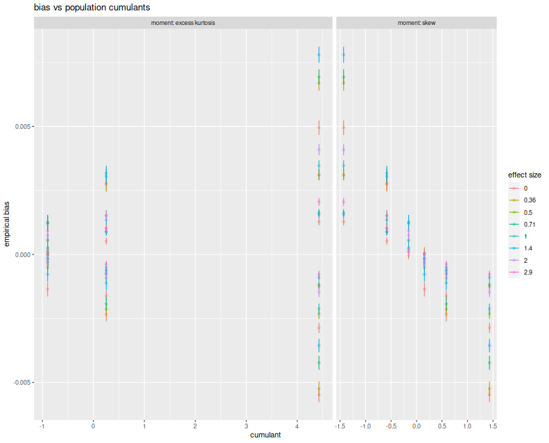
Here I plot the empirical average biases versus the population skew and the
population excess kurtosis. On the right facet we clearly see that Sharpe
bias is decreasing in population skew. The choices of $\alpha$ and
$\lambda$ here do not give symmetric and kurtotic distributions, so it
seems worthwhile to re-test this with returns drawn from, say, the $t$
distribution.
(The plot color corresponds to 'effect size',
which is $\sqrt{n}\zeta$, a unitless quantity, but which gives little
information in this plot.)
# plot empirical error vs cumulant.
library(ggplot2)
ph <- sumres %>%
    mutate(`effect size`=factor(signif(sqrt(n) * pzeta,digits=2))) %>%
    rename(`excess kurtosis`=exkurt) %>%
    tidyr::gather(key=moment,value=value,skew,`excess kurtosis`) %>%
    mutate(n=factor(n)) %>%
    ggplot(aes(x=value,y=mean_emp,color=`effect size`)) +
    geom_jitter(alpha=0.3) +
    geom_errorbar(aes(ymin=mean_emp - serr_emp,ymax=mean_emp + serr_emp)) +
    facet_grid(. ~ moment,labeller=label_both,scales='free',space='free') +
    labs(title='bias vs population cumulants',x='cumulant',y='empirical bias')
print(ph)
Here I plot the mean feasible and infeasible bias estimates against the
empirical biases, with different facets for $\alpha, \lambda, n$. Within
each facet there should be four populations, corresponding to the
Signal Noise ratio varying from 0 to $4$ annualized (yes, this is very high).
I plot horizontal error bars at 1 standard error, and the $y=x$ line.
There seems to be very little difference between the different estimators
of bias, and they all seem to be very close to the $y=x$ line to consider
them passable estimates of the bias.
# plot vs empirical error.
ph <- sumres %>%
    tidyr::gather(key=series,value=value,mean_bao,mean_thr,real_bias_skew,real_bias_bao) %>%
    ggplot(aes(x=mean_emp,y=value,color=series)) +
    geom_point() +
    facet_grid(n + alpha ~ lambda,labeller=label_both,scales='free',space='free') +
    geom_abline(intercept=0,slope=1,linetype=2,alpha=0.3) +
    geom_errorbarh(aes(xmin=mean_emp-serr_emp,xmax=mean_emp+serr_emp,height=.0005)) +
    theme(axis.text.x=element_text(angle=-45)) +
    labs(title='bias',x='empirical bias',y='approximations')
print(ph)
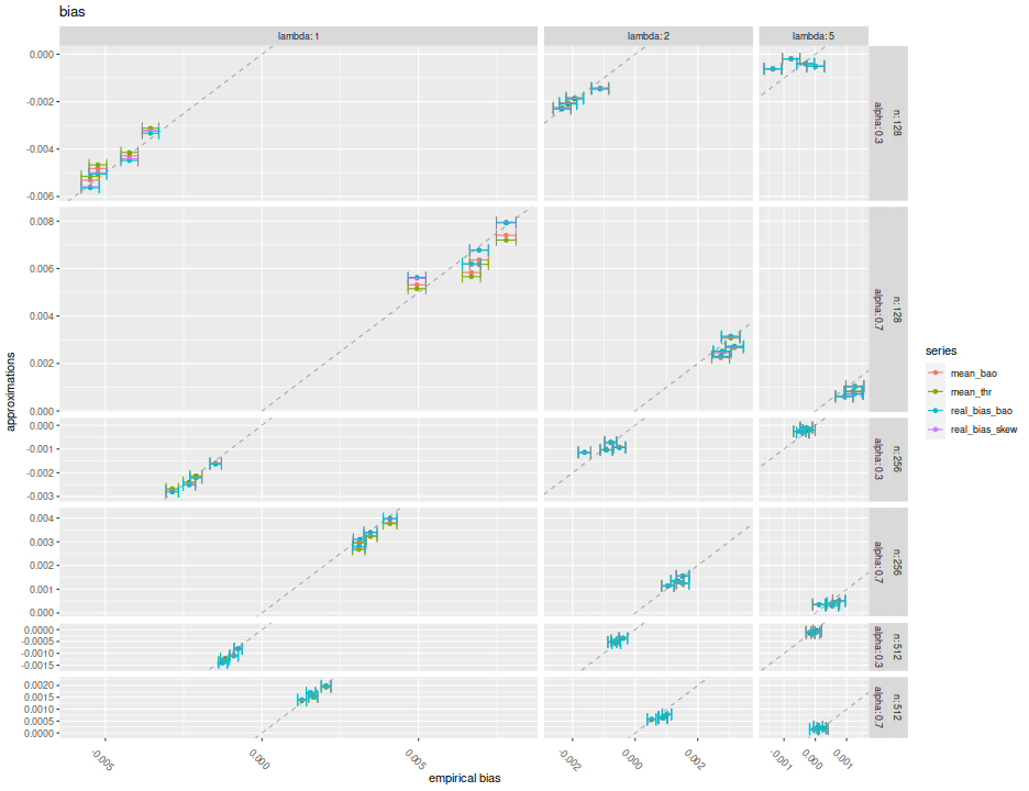
Both the formula given above and Bao's formula seem to capture the bias of the
Sharpe ratio in the simulations considered here. In their feasible forms,
neither of them seems seriously affected by estimation error of the higher
order cumulants, in expectation. I will recommend either of them, and hope to
include them as options in SharpeR.
Note, however, that for the purpose of hypothesis tests on the Signal Noise
ratio, say, that the bias is essentially $\operatorname{o}\left(n^{-1}\right)$
in the cumulants, but Mertens' correction to the standard error of the
Sharpe is $\operatorname{o}\left(n^{-1/2}\right)$. That is, I expect very
little to change in a hypothesis test by incorporating the bias term if
Mertens' correction is already being used. Moreover, I expect using the
bias term to have little improvement on the mean squared error,
especially versus the drawdown estimator.
Click to read and post comments
In a series of blog posts I have looked at Damien Challet's drawdown
estimator of the Signal to Noise ratio. My simulations
indicate that this estimator achieves its apparent efficiency at the cost
of some bias. Here I make a brief attempt at 'improving' the usual
moment-based estimator, the Sharpe ratio, by adding some extra terms.
If you want to play along at home, the rest of this blog post is
available as a jupyter notebook
off of a gist.
Let $\mu$, and $\sigma$ be the mean and standard deviation of the returns of an asset. Then $\zeta = \mu / \sigma$ is the "Signal to Noise Ratio" (SNR). Typically the SNR is estimated with the Sharpe Ratio, defined as $\hat{\zeta} = \hat{\mu} / \hat{\sigma}$, where $\hat{\mu}$ and $\hat{\sigma}$ are the vanilla sample estimates. Can we gain efficiency in the case where the returns have significant skew and kurtosis?
Here we consider an estimator of the form
$$
v = a_0 + \frac{a_1 + \left(1+a_2\right)\hat{\mu} + a_3 \hat{\mu}^2}{\hat{\sigma}} + a_4 \left(\frac{\hat{\mu}}{\hat{\sigma}}\right)^2.
$$
The Sharpe Ratio corresponds to $a_0 = a_1 = a_2 = a_3 = a_4 = 0$. Note that we were inspired by
Norman Johnson's work on t-tests under skewed distributions. Johnson considered a similar setup, but with only $a_1, a_2,$ and $a_3$ free, and was concerned with the problem of hypothesis testing on $\mu$.
Below, following Johnson, I will use the Cornish Fisher expansions of $\hat{\mu}$ and $\hat{\sigma}$ to approximate $v$ as a function of the first few cumulants of the distribution, and some normal variates. I will then compute the mean square error, $E\left[\left(v - \zeta\right)^2\right],$ and take its derivative with respect to $a_i$. Unfortunately, we will find that the first order conditions are solved by $a_i=0$, which is to say that the vanilla Sharpe has the lowest MSE of estimators of this kind. Our adventure will take us far, but we will return home empty handed.
We proceed.
# load what we need from sympy
from __future__ import division
from sympy import *
from sympy import Order
from sympy.assumptions.assume import global_assumptions
from sympy.stats import P, E, variance, Normal
init_printing()
nfactor = 4

# define some symbols.
a0, a1, a2, a3, a4 = symbols('a_0 a_1 a_2 a_3 a_4',real=True)
n, sigma = symbols('n \sigma',real=True,positive=True)
zeta, mu3, mu4 = symbols('\zeta \mu_3 \mu_4',real=True)
mu = zeta * sigma
We now express $\hat{\mu}$ and $\hat{\sigma}^2$ by the Cornish Fisher expansion. This is an expression of the distribution of a random variable in terms of its cumulants and a normal variate. The expansion is ordered in a way such that when applied to the mean of independent draws of a distribution, the terms are clustered by the order of $n$. The Cornish Fisher expansion also involves the Hermite polynomials. The expansions of $\hat{\mu}$ and $\hat{\sigma}^2$ are not independent. We follow Johnson in expression the correlation of normals and truncating:
# probabilist's hermite polynomials
def Hen(x,n):
    return (2**(-n/2) * hermite(n,x/sqrt(2)))

# this comes out of the wikipedia page:
h1 = lambda x : Hen(x,2) / 6
h2 = lambda x : Hen(x,3) / 24
h11 = lambda x : - (2 * Hen(x,3) + Hen(x,1)) / 36

# mu3 is the 3rd centered moment of x
gamma1 = (mu3 / (sigma**(3/2))) / sqrt(n)
gamma2 = (mu4 / (sigma**4)) / n

# grab two normal variates with correlation rho
# which happens to take value:
# rho = mu3 / sqrt(sigma**2 * (mu4 - sigma**4))
z1 = Normal('z_1',0,1)
z3 = Normal('z_3',0,1)
rho = symbols('\\rho',real=True)
z2 = rho * z1 + sqrt(1-rho**2)*z3

# this is out of Johnson, but we call it mu hat instead of x bar:
muhat = mu + (sigma/sqrt(n)) * (z1 + gamma1 * h1(z1) + gamma2 * h2(z1) + gamma1**2 * h11(z1))
muhat
$$\sigma \zeta + \frac{\sigma}{\sqrt{n}} \left(\frac{\mu_3^{2}}{\sigma^{3.0} n} \left(- 0.0392837100659193 \sqrt{2} z_{1}^{3} + 0.0982092751647983 \sqrt{2} z_{1}\right)\
+ \frac{\mu_3}{\sigma^{1.5} \sqrt{n}} \left(0.166666666666667 z_{1}^{2} - 0.166666666666667\right) \
+ \frac{\mu_4}{\sigma^{4} n} \left(0.0294627825494395 \sqrt{2} z_{1}^{3} - 0.0883883476483184 \sqrt{2} z_{1}\right) + z_{1}\right)$$
addo = sqrt((mu4 - sigma**4) / (n * sigma**4)) * z2
# this is s^2 in Johnson:
sighat2 = (sigma**2) * (1 + addo)
# use Taylor's theorem to express sighat^-1:
invs = (sigma**(-1)) * (1 - (1/(2*sigma)) * addo)
invs
$$\frac{1}{\sigma} \left(1 - \frac{\sqrt{\mu_4 - \sigma^{4}}}{2 \sigma^{3} \sqrt{n}} \left(\rho z_{1} + \sqrt{- \rho^{2} + 1} z_{3}\right)\right)$$
# the new statistic; it is v = part1 + part2 + part3
part1 = a0
part2 = (a1 + (1+a2)*muhat + a3 * muhat**2) * invs
part3 = a4 * (muhat*invs)**2

v = part1 + part2 + part3
v
$$a_{0} + \frac{1}{\sigma} \left(1 - \frac{\sqrt{\mu_4 - \sigma^{4}}}{2 \sigma^{3} \sqrt{n}} \left(\rho z_{1} + \sqrt{- \rho^{2} + 1} z_{3}\right)\right) \left(a_{1} \
+ a_{3} \left(\sigma \zeta + \frac{\sigma}{\sqrt{n}} \left(\frac{\mu_3^{2}}{\sigma^{3.0} n} \left(- 0.0392837100659193 \sqrt{2} z_{1}^{3} + 0.0982092751647983 \sqrt{2} z_{1}\right) \
+ \frac{\mu_3}{\sigma^{1.5} \sqrt{n}} \left(0.166666666666667 z_{1}^{2} - 0.166666666666667\right) \
+ \frac{\mu_4}{\sigma^{4} n} \left(0.0294627825494395 \sqrt{2} z_{1}^{3} - 0.0883883476483184 \sqrt{2} z_{1}\right) + z_{1}\right)\right)^{2} \
+ \left(a_{2} + 1\right) \left(\sigma \zeta + \frac{\sigma}{\sqrt{n}} \left(\frac{\mu_3^{2}}{\sigma^{3.0} n} \left(- 0.0392837100659193 \sqrt{2} z_{1}^{3} + 0.0982092751647983 \sqrt{2} z_{1}\right) \
+ \frac{\mu_3}{\sigma^{1.5} \sqrt{n}} \left(0.166666666666667 z_{1}^{2} - 0.166666666666667\right) \
+ \frac{\mu_4}{\sigma^{4} n} \left(0.0294627825494395 \sqrt{2} z_{1}^{3} - 0.0883883476483184 \sqrt{2} z_{1}\right) + z_{1}\right)\right)\right) \
+ \frac{a_{4}}{\sigma^{2}} \left(1 - \frac{\sqrt{\mu_4 - \sigma^{4}}}{2 \sigma^{3} \sqrt{n}} \left(\rho z_{1} + \sqrt{- \rho^{2} + 1} z_{3}\right)\right)^{2} \left(\sigma \zeta \
+ \frac{\sigma}{\sqrt{n}} \left(\frac{\mu_3^{2}}{\sigma^{3.0} n} \left(- 0.0392837100659193 \sqrt{2} z_{1}^{3} + 0.0982092751647983 \sqrt{2} z_{1}\right) \
+ \frac{\mu_3}{\sigma^{1.5} \sqrt{n}} \left(0.166666666666667 z_{1}^{2} - 0.166666666666667\right) \
+ \frac{\mu_4}{\sigma^{4} n} \left(0.0294627825494395 \sqrt{2} z_{1}^{3} - 0.0883883476483184 \sqrt{2} z_{1}\right) + z_{1}\right)\right)^{2}$$
That's a bit hairy. Here I truncate that statistic in $n$. This was hard for me to figure out in sympy, so I took a limit. (I like how 'oo' is infinity in sympy.)
#show nothing
v_0 = limit(v,n,oo)
v_05 = v_0 + (limit(sqrt(n) * (v - v_0),n,oo) / sqrt(n))
v_05
$$\frac{1}{\sigma^{17.0} \sqrt{n}} \left(- 0.5 \rho \sigma^{13.0} a_{1} \sqrt{\mu_4 - \sigma^{4}} z_{1} - 1.0 \rho \sigma^{14.0} \zeta^{2} a_{4} \sqrt{\mu_4 - \sigma^{4}} z_{1} - 0.5 \rho \sigma^{14.0} \zeta a_{2} \sqrt{\mu_4 - \sigma^{4}} z_{1} \
- 0.5 \rho \sigma^{14.0} \zeta \sqrt{\mu_4 - \sigma^{4}} z_{1} - 0.5 \rho \sigma^{15.0} \zeta^{2} a_{3} \sqrt{\mu_4 - \sigma^{4}} z_{1} - 0.5 \sigma^{13.0} a_{1} \sqrt{\mu_4 - \sigma^{4}} \sqrt{- \rho^{2} + 1} z_{3} \
- 1.0 \sigma^{14.0} \zeta^{2} a_{4} \sqrt{\mu_4 - \sigma^{4}} \sqrt{- \rho^{2} + 1} z_{3} - 0.5 \sigma^{14.0} \zeta a_{2} \sqrt{\mu_4 - \sigma^{4}} \sqrt{- \rho^{2} + 1} z_{3} \
- 0.5 \sigma^{14.0} \zeta \sqrt{\mu_4 - \sigma^{4}} \sqrt{- \rho^{2} + 1} z_{3} - 0.5 \sigma^{15.0} \zeta^{2} a_{3} \sqrt{\mu_4 - \sigma^{4}} \sqrt{- \rho^{2} + 1} z_{3} + 2.0 \sigma^{17.0} \zeta a_{4} z_{1} \
+ 1.0 \sigma^{17.0} a_{2} z_{1} + 1.0 \sigma^{17.0} z_{1} + 2.0 \sigma^{18.0} \zeta a_{3} z_{1}\right) + \frac{1}{\sigma} \left(\sigma^{2} \zeta^{2} a_{3} \
+ \sigma \zeta^{2} a_{4} + \sigma \zeta a_{2} + \sigma \zeta + \sigma a_{0} + a_{1}\right)$$
Now we define the error as $v - \zeta$ and compute the approximate bias and variance of the error. We sum the variance and squared bias to get mean square error.
staterr = v_05 - zeta
# mean squared error of the statistic v, is
# MSE = E((newstat - zeta)**2)
# this is too slow, though, so evaluate them separately instead:
bias = E(staterr)
simplify(bias)
$$\sigma \zeta^{2} a_{3} + \zeta^{2} a_{4} + \zeta a_{2} + a_{0} + \frac{a_{1}}{\sigma}$$
# variance of the error:
varerr = variance(staterr)
MSE = (bias**2) + varerr
collect(MSE,n)
$$\left(- \zeta + \frac{1}{\sigma} \left(\sigma^{2} \zeta^{2} a_{3} + \sigma \zeta^{2} a_{4} + \sigma \zeta a_{2} + \sigma \zeta + \sigma a_{0} + a_{1}\right)\right)^{2} \
+ \frac{1}{n} \left(\frac{0.25 \mu_4}{\sigma^{8.0}} a_{1}^{2} + \frac{1.0 \mu_4}{\sigma^{7.0}} \zeta^{2} a_{1} a_{4} + \frac{0.5 \mu_4}{\sigma^{7.0}} \zeta a_{1} a_{2}
+ \frac{0.5 \mu_4}{\sigma^{7.0}} \zeta a_{1} + \frac{1.0 \mu_4}{\sigma^{6.0}} \zeta^{4} a_{4}^{2} + \frac{1.0 \mu_4}{\sigma^{6.0}} \zeta^{3} a_{2} a_{4} \
+ \frac{1.0 \mu_4}{\sigma^{6.0}} \zeta^{3} a_{4} + \frac{0.5 \mu_4}{\sigma^{6.0}} \zeta^{2} a_{1} a_{3} + \frac{0.25 \mu_4}{\sigma^{6.0}} \zeta^{2} a_{2}^{2}
+ \frac{0.5 \mu_4}{\sigma^{6.0}} \zeta^{2} a_{2} + \frac{0.25 \mu_4}{\sigma^{6.0}} \zeta^{2} + \frac{1.0 \mu_4}{\sigma^{5.0}} \zeta^{4} a_{3} a_{4} \
+ \frac{0.5 \mu_4}{\sigma^{5.0}} \zeta^{3} a_{2} a_{3} + \frac{0.5 \mu_4}{\sigma^{5.0}} \zeta^{3} a_{3} + \frac{0.25 \mu_4}{\sigma^{4.0}} \zeta^{4} a_{3}^{2}
- \frac{2.0 \rho}{\sigma^{4.0}} \zeta a_{1} a_{4} \sqrt{\mu_4 - \sigma^{4}} - \frac{1.0 \rho}{\sigma^{4.0}} a_{1} a_{2} \sqrt{\mu_4 - \sigma^{4}} \
- \frac{1.0 \rho}{\sigma^{4.0}} a_{1} \sqrt{\mu_4 - \sigma^{4}} - \frac{4.0 \rho}{\sigma^{3.0}} \zeta^{3} a_{4}^{2} \sqrt{\mu_4 - \sigma^{4}}
- \frac{4.0 \rho}{\sigma^{3.0}} \zeta^{2} a_{2} a_{4} \sqrt{\mu_4 - \sigma^{4}} - \frac{4.0 \rho}{\sigma^{3.0}} \zeta^{2} a_{4} \sqrt{\mu_4 - \sigma^{4}} \
- \frac{2.0 \rho}{\sigma^{3.0}} \zeta a_{1} a_{3} \sqrt{\mu_4 - \sigma^{4}} - \frac{1.0 \rho}{\sigma^{3.0}} \zeta a_{2}^{2} \sqrt{\mu_4 - \sigma^{4}}
- \frac{2.0 \rho}{\sigma^{3.0}} \zeta a_{2} \sqrt{\mu_4 - \sigma^{4}} - \frac{1.0 \rho}{\sigma^{3.0}} \zeta \sqrt{\mu_4 - \sigma^{4}} \
- \frac{6.0 \rho}{\sigma^{2.0}} \zeta^{3} a_{3} a_{4} \sqrt{\mu_4 - \sigma^{4}} - \frac{3.0 \rho}{\sigma^{2.0}} \zeta^{2} a_{2} a_{3} \sqrt{\mu_4 - \sigma^{4}}
- \frac{3.0 \rho}{\sigma^{2.0}} \zeta^{2} a_{3} \sqrt{\mu_4 - \sigma^{4}} - \frac{2.0 \rho}{\sigma^{1.0}} \zeta^{3} a_{3}^{2} \sqrt{\mu_4 - \sigma^{4}} \
- \frac{0.25 a_{1}^{2}}{\sigma^{4.0}} - \frac{1.0 a_{1}}{\sigma^{3.0}} \zeta^{2} a_{4} - \frac{0.5 \zeta}{\sigma^{3.0}} a_{1} a_{2}
- \frac{0.5 \zeta}{\sigma^{3.0}} a_{1} - \frac{1.0 \zeta^{4}}{\sigma^{2.0}} a_{4}^{2} - \frac{1.0 a_{2}}{\sigma^{2.0}} \zeta^{3} a_{4} \
- \frac{1.0 a_{4}}{\sigma^{2.0}} \zeta^{3} - \frac{0.5 a_{1}}{\sigma^{2.0}} \zeta^{2} a_{3} - \frac{0.25 \zeta^{2}}{\sigma^{2.0}} a_{2}^{2}
- \frac{0.5 a_{2}}{\sigma^{2.0}} \zeta^{2} - \frac{0.25 \zeta^{2}}{\sigma^{2.0}} - \frac{1.0 a_{3}}{\sigma^{1.0}} \zeta^{4} a_{4} \
- \frac{0.5 a_{2}}{\sigma^{1.0}} \zeta^{3} a_{3} - \frac{0.5 a_{3}}{\sigma^{1.0}} \zeta^{3} + 8.0 \sigma^{1.0} \zeta^{2} a_{3} a_{4}
+ 4.0 \sigma^{1.0} \zeta a_{2} a_{3} + 4.0 \sigma^{1.0} \zeta a_{3} + 4.0 \sigma^{2.0} \zeta^{2} a_{3}^{2} \
- 0.25 \zeta^{4} a_{3}^{2} + 4.0 \zeta^{2} a_{4}^{2} + 4.0 \zeta a_{2} a_{4} + 4.0 \zeta a_{4} + 1.0 a_{2}^{2} + 2.0 a_{2} + 1.0\right)$$
That's really involved, and finding the derivative will be ugly. Instead we truncate at $n^{-1}$, which leaves us terms constant in $n$. Looking above, you will see that removing terms in $n^{-1}$ leaves some quantity squared. That is what we will minimize. The way forward is fairly clear from here.
# truncate!
MSE_0 = limit(collect(MSE,n),n,oo)
MSE_1 = MSE_0 + (limit(n * (MSE - MSE_0),n,oo)/n)
MSE_0
$$\frac{1}{\sigma^{2}} \left(\sigma^{4} \zeta^{4} a_{3}^{2} + 2 \sigma^{3} \zeta^{4} a_{3} a_{4} + 2 \sigma^{3} \zeta^{3} a_{2} a_{3} + 2 \sigma^{3} \zeta^{2} a_{0} a_{3} + \sigma^{2} \zeta^{4} a_{4}^{2} + 2 \sigma^{2} \zeta^{3} a_{2} a_{4} + 2 \sigma^{2} \zeta^{2} a_{0} a_{4} \
+ 2 \sigma^{2} \zeta^{2} a_{1} a_{3} + \sigma^{2} \zeta^{2} a_{2}^{2} + 2 \sigma^{2} \zeta a_{0} a_{2} + \sigma^{2} a_{0}^{2} + 2 \sigma \zeta^{2} a_{1} a_{4} + 2 \sigma \zeta a_{1} a_{2} + 2 \sigma a_{0} a_{1} + a_{1}^{2}\right)$$
Now we take the derivative of the Mean Square Error with respect to the $a_i$. In each case we will get an equation linear in all the $a_i$. The first order condition, which corresponds to minimizing the MSE, occurs for $a_i=0$.
# a_0
simplify(diff(MSE_0,a0))
$$2 \sigma \zeta^{2} a_{3} + 2 \zeta^{2} a_{4} + 2 \zeta a_{2} + 2 a_{0} + \frac{2 a_{1}}{\sigma}$$
# a_1
simplify(diff(MSE_0,a1))
$$2 \zeta^{2} a_{3} + \frac{2 a_{4}}{\sigma} \zeta^{2} + \frac{2 \zeta}{\sigma} a_{2} + \frac{2 a_{0}}{\sigma} + \frac{2 a_{1}}{\sigma^{2}}$$
# a_2
simplify(diff(MSE_0,a2))
$$\frac{2 \zeta}{\sigma} \left(\sigma^{2} \zeta^{2} a_{3} + \sigma \zeta^{2} a_{4} + \sigma \zeta a_{2} + \sigma a_{0} + a_{1}\right)$$
# a_3
simplify(diff(MSE_0,a3))
$$2 \zeta^{2} \left(\sigma^{2} \zeta^{2} a_{3} + \sigma \zeta^{2} a_{4} + \sigma \zeta a_{2} + \sigma a_{0} + a_{1}\right)$$
# a_4
simplify(diff(MSE_0,a4))
$$\frac{2 \zeta^{2}}{\sigma} \left(\sigma^{2} \zeta^{2} a_{3} + \sigma \zeta^{2} a_{4} + \sigma \zeta a_{2} + \sigma a_{0} + a_{1}\right)$$
To recap, the minimal MSE occurs for $a_0 = a_1 = a_2 = a_3 = a_4 = 0$. We must try another approach.
Click to read and post comments