The Sharpe Ratio is Biased
That the Sharpe ratio is biased is not unknown; this was established for Gaussian returns by Miller and Gehr in 1978. In the non-Gaussian case, the analyses of Jobson and Korkie (1981), Lo (2002), and Mertens (2002) have focused on the asymptotic distribution of the Sharpe ratio, via the Central Limit Theorem and the delta method. These techniques generally establish that the estimator is asymptotically unbiased, with some specified asymptotic variance.
The lack of asymptotic bias is not terribly comforting in our world of finite, sometimes small, sample sizes. Moreover, the finite sample bias of the Sharpe ratio might be geometric, which means that we could arrive at an estimator with smaller Mean Square Error (MSE), by dividing the Sharpe by some quantity. Finding the bias of the Sharpe seems like a straightforward application of Taylor's theorem. First we write $$ \hat{\sigma}^2 = \sigma^2 \left(1 + \frac{\hat{\sigma}^2 - \sigma^2}{\sigma^2}\right) $$ We can think of $\epsilon = \frac{\hat{\sigma^2} - \sigma^2}{\sigma^2}$ as the error, when we perform a Taylor expansion of $x^{-1/2}$ around $1$. That expansion is $$ \left(\sigma^2 \left(1 + \epsilon\right)\right)^{-1/2} \approx \sigma^{-1}\left(1 - \frac{1}{2}\epsilon + \frac{3}{8}\epsilon^2 + \ldots \right) $$ We can use linearity of expectation to get the expectation of the Sharpe ratio (which I denote $\hat{\zeta}$) as follows: $$ \operatorname{E}\left[\hat{\zeta}\right] = \zeta\left(1 - \frac{1}{2}\operatorname{E}\left[\hat{\mu} \frac{\hat{\sigma}^2 - \sigma^2}{\sigma^2} \right] + \frac{3}{8} \operatorname{E}\left[ \hat{\mu} \left(\frac{\hat{\sigma}^2 - \sigma^2}{\sigma^2} \right)^2 \right] + \ldots \right) $$ After some ugly computations, we arrive at $$ \operatorname{E}\left[\hat{\zeta}\right] \approx \left(1 + \frac{3}{4n} + \frac{3\kappa}{8n}\right) \zeta - \frac{1}{2n}s + \operatorname{o}\left(n^{-3/2}\right). $$
As the saying goes, a week of scratching out equations can save you an hour in the library (or 5 minutes on google). This computation has been performed before (and more importantly, vetted by an editor). The paper I should have read (and should have read a long time ago) is the 2009 paper by Yong Bao, Estimation Risk-Adjusted Sharpe Ratio and Fund Performance Ranking Under a General Return Distribution. Bao uses what he calls a 'Nagar-type expansion' (I am not familiar with the reference) by essentially splitting $\hat{\mu}$ into $\mu + \left(\hat{\mu} - \mu\right)$, then separating terms based on whether they contain $\hat{\mu}$ to arrive at an estimate with more terms than shown above, but greater accuracy, a $\operatorname{o}\left(n^{-2}\right)$ error.
(Bao goes on to consider a 'double Sharpe ratio', following Vinod and Morey. The double Sharpe ratio is a Studentized Sharpe ratio: the Sharpe minus it's bias, then divided by its standard error. This is the Wald statistic for the implicit hypothesis test that the Signal-Noise ratio (i.e. the population Sharpe ratio) is equal to zero. It is not clear why zero is chosen as the null value.)
Yong Bao was kind enough to share his Gauss code. I have translated it into R, hopefully without error. Below I run some simulations with returns drawn from the 'Asymmetric Power Distribution' (APD) with varying values of $n$, $\zeta$, $\alpha$ and $\lambda$. For each setting of the parameters, I perform $10^5$ simulations, then compute the bias of the sample Sharpe ratio, then I use Bao's formula and the simplified formula above, but plugging in sample estimates of the Sharpe, skew, kurtosis, and so on to arrive at feasible estimates. I then compute, over the 100K simulations, the mean empirical bias, and the mean feasible estimators. I then use the two formulae with the population values to get infeasible biases.
suppressMessages({
  library(dplyr)
  library(tidyr)
  library(tibble)
  library(ggplot2)
  library(future.apply)
})
# /* k-statistic, see Kendall's Advanced Theory of Statistics */
.kstat <- function(x) {
    # note we can make this faster because we have subtracted off the mean
    # so s[1]=0 identically, but don't bother for now.
    n <- length(x)
    s <- unlist(lapply(1:6,function(iii) { sum(x^iii) }))
    nn <- n^(1:6)
    nd <- exp(lfactorial(n) - lfactorial(n-(1:6)))
    k <- rep(0,6)
    k[1] <- s[1]/n;
    k[2] <- (n*s[2]-s[1]^2)/nd[2];
    k[3] <- (nn[2]*s[3]-3*n*s[2]*s[1]+2*s[1]^3)/nd[3]
    k[4] <- ((nn[3]+nn[2])*s[4]-4*(nn[2]+n)*s[3]*s[1]-3*(nn[2]-n)*s[2]^2 +12*n*s[2]*s[1]^2-6*s[1]^4)/nd[4];
    k[5] <- ((nn[4]+5*nn[3])*s[5]-5*(nn[3]+5*nn[2])*s[4]*s[1]-10*(nn[3]-nn[2])*s[3]*s[2]
                     +20*(nn[2]+2*n)*s[3]*s[1]^2+30*(nn[2]-n)*s[2]^2*s[1]-60*n*s[2]*s[1]^3 +24*s[1]^5)/nd[5];
    k[6] <- ((nn[5]+16*nn[4]+11*nn[3]-4*nn[2])*s[6]
                    -6*(nn[4]+16*nn[3]+11*nn[2]-4*n)*s[5]*s[1]
                    -15*n*(n-1)^2*(n+4)*s[4]*s[2]-10*(nn[4]-2*nn[3]+5*nn[2]-4*n)*s[3]^2
                    +30*(nn[3]+9*nn[2]+2*n)*s[4]*s[1]^2+120*(nn[3]-n)*s[3]*s[2]*s[1]
                    +30*(nn[3]-3*nn[2]+2*n)*s[2]^3-120*(nn[2]+3*n)*s[3]*s[1]^3
                    -270*(nn[2]-n)*s[2]^2*s[1]^2+360*n*s[2]*s[1]^4-120*s[1]^6)/nd[6];

    k
}
# sample gammas from observation;
# first value is mean, second is variance, then standardized 3 through 6
# moments
some_gams <- function(y) {
    mu <- mean(y)
    x <- y - mu
    k <- .kstat(x)
    retv <- c(mu,k[2],k[3:6] / (k[2] ^ ((3:6)/2)))
    retv
}
# /* Simulate Standadized APD */
.deltafn <- function(alpha,lambda) {
    2*alpha^lambda*(1-alpha)^lambda/(alpha^lambda+(1-alpha)^lambda)
}
apdmoment <- function(alpha,lambda,r) {
    delta <- .deltafn(alpha,lambda);
    m <- gamma((1+r)/lambda)*((1-alpha)^(1+r)+(-1)^r*alpha^(1+r));
    m <- m/gamma(1/lambda);
    m <- m/(delta^(r/lambda));
    m
}
# variates from the APD;
.rapd <- function(n,alpha,lambda,delta,m1,m2) {
    W <- rgamma(n, scale=1, shape=1/lambda)
    V <- (W/delta)^(1/lambda)
    e <- runif(n)
    S <- -1*(e<=alpha)+(e>alpha)
    U <- -alpha*(V*(S<=0))+(1-alpha)*(V*(S>0))
    Z <- (U-m1)/sqrt(m2-m1^2); # /* Standardized APD */
}
# to get APD distributions use this:
#rapd <- function(n,alpha,lambda) {
#   delta <- .deltafn(alpha,lambda)
#   # /* APD moments about zero */
#   m1 <- apdmoment(alpha=alpha,lambda=lambda,1);
#   m2 <- apdmoment(alpha=alpha,lambda=lambda,2);
#   Z <- .rapd(n,alpha=alpha,lambda=lambda,delta=delta,m1=m1,m2=m2)
#}

# /* From uncentered moment m to centered moment mu */
.m_to_mu <- function(m) {
    n <- length(m)
    mu <- m
    for (iii in 2:n) {
            for (jjj in 1:iii) {
                    if (jjj<iii) {
                            mu[iii] <- mu[iii] + choose(iii,jjj) * m[iii-jjj]*(-m[1])^jjj;
                    } else {
                            mu[iii] <- mu[iii] + choose(iii,jjj) * (-m[1])^jjj;
                    }
            }
    }
    mu
}

# true centered moments of the APD distribution
.apd_centered <- function(alpha,lambda) {
    m <- unlist(lapply(1:6,apdmoment,alpha=alpha,lambda=lambda))
    mu <- .m_to_mu(m)
}
# true standardized moments of the APD distribution
.apd_standardized <- function(alpha,lambda) {
    k <- .apd_centered(alpha,lambda)
    retv <- c(1,1,k[3:6] / (k[2] ^ ((3:6)/2)))
}
# true APD cumulants: skew, excess kurtosis, ...
.apd_r <- function(alpha,lambda) {
    mustandardized <- .apd_standardized(alpha,lambda)
    r <- rep(0,4)
    r[1] <- mustandardized[3]
    r[2] <- mustandardized[4]-3
    r[3] <- mustandardized[5]-10*r[1]
    r[4] <- mustandardized[6]-15*r[2]-10*r[1]^2-15
    r
}
# Bao's Bias function;
# use this in the feasible and infeasible.
.bias2 <- function(TT,S,r) {
    retv <- 3*S/4/TT+49*S/32/TT^2-r[1]*(1/2/TT+3/8/TT^2)+S*r[2]*(3/8/TT-15/32/TT^2) +3*r[3]/8/TT^2-5*S*r[4]/16/TT^2-5*S*r[1]^2/4/TT^2+105*S*r[2]^2/128/TT^2-15*r[1]*r[2]/16/TT^2;
}
# one simulation.
onesim <- function(n,pzeta,alpha,lambda,delta,m1,m2,...) {
  x <- pzeta + .rapd(n=n,alpha=alpha,lambda=lambda,delta=delta,m1=m1,m2=m2)
    rhat <- some_gams(x)
    Shat <- rhat[1] / sqrt(rhat[2])
    emp_bias <- Shat - pzeta
    # feasible bias estimation
    feas_bias_skew <- (3/(8*n)) * (2 + rhat[4]) * Shat - (1/(2*n)) * rhat[3]
    feas_bias_bao <- .bias2(TT=n,S=Shat,r=rhat[3:6])
    cbind(pzeta,emp_bias,feas_bias_skew,feas_bias_bao)
}
# many sims.
repsim <- function(nrep,n,pzeta,alpha,lambda,delta,m1,m2) {
  jumble <- replicate(nrep,onesim(n=n,pzeta=pzeta,alpha=alpha,lambda=lambda,delta=delta,m1=m1,m2=m2))
  retv <- aperm(jumble,c(1,3,2))
  dim(retv) <- c(nrep * length(pzeta),dim(jumble)[2])
  colnames(retv) <- colnames(jumble)
  invisible(as.data.frame(retv))
}
manysim <- function(nrep,n,pzeta,alpha,lambda,nnodes=7) {
    delta <- .deltafn(alpha,lambda)
    # /* APD moments about zero */
    m1 <- apdmoment(alpha=alpha,lambda=lambda,1);
    m2 <- apdmoment(alpha=alpha,lambda=lambda,2);

  if (nrep > 2*nnodes) {
    # do in parallel.
    nper <- table(1 + ((0:(nrep-1) %% nnodes)))
        plan(multisession, workers = 7)
    retv <- future_lapply(nper,FUN=function(aper) repsim(nrep=aper,n=n,pzeta=pzeta,alpha=alpha,lambda=lambda,delta=delta,m1=m1,m2=m2)) %>%
      bind_rows()
        plan(sequential)
  } else {
        retv <- repsim(nrep=nrep,n=n,pzeta=pzeta,alpha=alpha,lambda=lambda,delta=delta,m1=m1,m2=m2)
  }
  retv
}

ope <- 252
pzetasq <- c(0,1/4,1,4) / ope
pzeta <- sqrt(pzetasq)

apd_param <- tibble::tribble(~dgp,   ~alpha,  ~lambda,
                                                         'dgp7',    0.3,        1,
                                                         'dgp8',    0.3,        2,
                                                         'dgp9',    0.3,        5,
                                                         'dgp10',   0.7,        1,
                                                         'dgp11',   0.7,        2,
                                                         'dgp12',   0.7,        5)

params <- tidyr::crossing(tibble::tribble(~n,128,256,512),
                          tibble::tibble(pzeta=pzeta),
                                                    apd_param)

# run a bunch; on my machine, with 8 cores,
# 5000 takes ~68 seconds
#  1e4 takes ~2 minutes.
#  1e5 should take 20?
nrep <- 1e5
set.seed(1234)
system.time({
results <- params %>%
  group_by(n,pzeta,dgp,alpha,lambda) %>%
    summarize(sims=list(manysim(nrep=nrep,nnodes=8,
                                pzeta=pzeta,n=n,alpha=alpha,lambda=lambda))) %>%
  ungroup() %>%
  tidyr::unnest() %>%
  dplyr::select(-pzeta1)
})
   user  system elapsed
 36.233   1.624 598.707
# pop moment/cumulant function
pop_moments <- function(pzeta,alpha,lambda) {
    rfoo <- .apd_r(alpha,lambda)
    data_frame(mean=pzeta,var=1,skew=rfoo[1],exkurt=rfoo[2])
}
# Bao bias function
pop_bias_bao <- function(n,pzeta,alpha,lambda) {
    rfoo <- .apd_r(alpha,lambda)
    rhat <- c(pzeta,1,rfoo)
    retv <- .bias2(TT=n,S=pzeta,r=rhat[3:6])
}
# attach population values and bias estimates
parres <- params %>%
    group_by(n,pzeta,dgp,alpha,lambda) %>%
        mutate(foo=list(pop_moments(pzeta,alpha,lambda))) %>%
    ungroup() %>%
    unnest() %>%
    group_by(n,pzeta,dgp,alpha,lambda) %>%
        mutate(real_bias_skew=(3/(8*n)) * (2 + exkurt) * pzeta - (1/(2*n)) * skew,
                     real_bias_bao =pop_bias_bao(n,pzeta,alpha,lambda)) %>%
    ungroup()
# put them all together
sumres <- results %>%
  group_by(dgp,pzeta,n,alpha,lambda) %>%
        summarize(mean_emp=mean(emp_bias),
                            serr_emp=sd(emp_bias) / sqrt(n()),
                            mean_bao=mean(feas_bias_bao),
                            mean_thr=mean(feas_bias_skew)) %>%
    ungroup() %>%
    left_join(parres,by=c('dgp','n','pzeta','alpha','lambda'))
# done
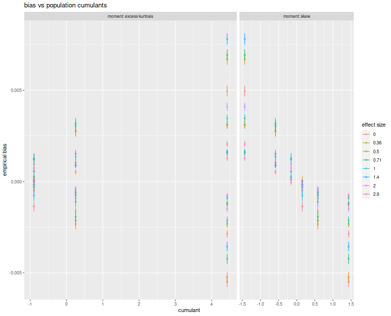
Here I plot the empirical average biases versus the population skew and the population excess kurtosis. On the right facet we clearly see that Sharpe bias is decreasing in population skew. The choices of $\alpha$ and $\lambda$ here do not give symmetric and kurtotic distributions, so it seems worthwhile to re-test this with returns drawn from, say, the $t$ distribution. (The plot color corresponds to 'effect size', which is $\sqrt{n}\zeta$, a unitless quantity, but which gives little information in this plot.)
# plot empirical error vs cumulant.
library(ggplot2)
ph <- sumres %>%
    mutate(`effect size`=factor(signif(sqrt(n) * pzeta,digits=2))) %>%
    rename(`excess kurtosis`=exkurt) %>%
    tidyr::gather(key=moment,value=value,skew,`excess kurtosis`) %>%
    mutate(n=factor(n)) %>%
    ggplot(aes(x=value,y=mean_emp,color=`effect size`)) +
    geom_jitter(alpha=0.3) +
    geom_errorbar(aes(ymin=mean_emp - serr_emp,ymax=mean_emp + serr_emp)) +
    facet_grid(. ~ moment,labeller=label_both,scales='free',space='free') +
    labs(title='bias vs population cumulants',x='cumulant',y='empirical bias')
print(ph)
Here I plot the mean feasible and infeasible bias estimates against the empirical biases, with different facets for $\alpha, \lambda, n$. Within each facet there should be four populations, corresponding to the Signal Noise ratio varying from 0 to $4$ annualized (yes, this is very high). I plot horizontal error bars at 1 standard error, and the $y=x$ line. There seems to be very little difference between the different estimators of bias, and they all seem to be very close to the $y=x$ line to consider them passable estimates of the bias.
# plot vs empirical error.
ph <- sumres %>%
    tidyr::gather(key=series,value=value,mean_bao,mean_thr,real_bias_skew,real_bias_bao) %>%
    ggplot(aes(x=mean_emp,y=value,color=series)) +
    geom_point() +
    facet_grid(n + alpha ~ lambda,labeller=label_both,scales='free',space='free') +
    geom_abline(intercept=0,slope=1,linetype=2,alpha=0.3) +
    geom_errorbarh(aes(xmin=mean_emp-serr_emp,xmax=mean_emp+serr_emp,height=.0005)) +
    theme(axis.text.x=element_text(angle=-45)) +
    labs(title='bias',x='empirical bias',y='approximations')
print(ph)
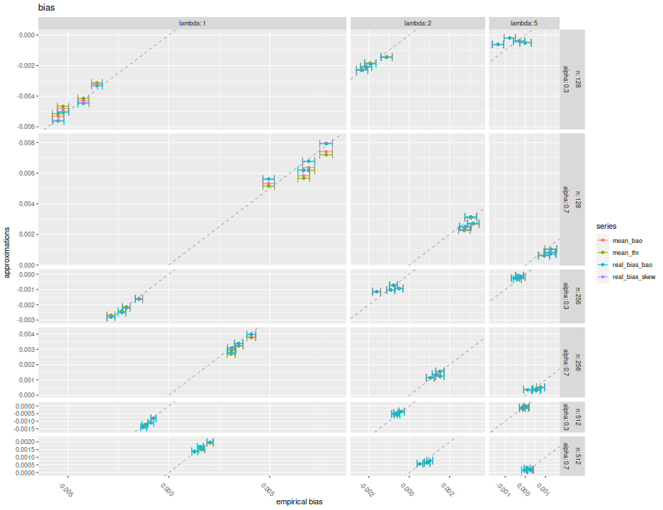
Both the formula given above and Bao's formula seem to capture the bias of the
Sharpe ratio in the simulations considered here. In their feasible forms,
neither of them seems seriously affected by estimation error of the higher
order cumulants, in expectation. I will recommend either of them, and hope to
include them as options in SharpeR.
Note, however, that for the purpose of hypothesis tests on the Signal Noise ratio, say, that the bias is essentially $\operatorname{o}\left(n^{-1}\right)$ in the cumulants, but Mertens' correction to the standard error of the Sharpe is $\operatorname{o}\left(n^{-1/2}\right)$. That is, I expect very little to change in a hypothesis test by incorporating the bias term if Mertens' correction is already being used. Moreover, I expect using the bias term to have little improvement on the mean squared error, especially versus the drawdown estimator.
Click to read and post comments