Conditional Inference Under Normal Skill and Luck
In a previous blog post I considered the "deflated Sharpe ratio" of Bailey and López de Prado and found it quite lacking: it comes with zero theoretical justification and fails to do anything sensible in practice. Here I consider a simple conditional estimator for the problem targeted by the deflated Sharpe ratio, one which actually exhibits good coverage.
We start from the same setup as the deflated Sharpe ratio: historical performance of a large number of strategies. The historical performance is the sum of skill and luck, both of which are normally distributed. (The normality of luck is a simplification we ignore for this blog post.) One selects the strategy with the best in-sample performance, then performs inference on the skill of that strategy. In this case the skill is population Sharpe ratio, while the in-sample performance is the sample Sharpe ratio. Again, you want a strategy with high skill, but can only select on skill plus luck.
In our case the luck is the noise of the in-sample Sharpe ratio around the signal-noise ratio. The magnitude of this noise is controlled mostly by the length of the backtest period, and is approximately $1/T$ where $T$ days of backtested returns are observed. So we suppose that the skill of the $i$th strategy, $\mu_i$ is normally distributed: $$ \mu_i \sim \mathcal{N}\left(\mu, \sigma^2_s\right). $$ We then observe the in-sample performance $x_i$ which is the sum of $\mu_i$ and a normal error: $$ \left(x_i - \mu_i\right) \sim \mathcal{N}\left(0, \sigma^2_l\right). $$ We assume that the $\left\{x_i, x_i-\mu_i\right\}$ are all independent of each other.
We write the vector of the $x_i, \mu_i$ as a bivariate normal: $$ \left[\begin{array}{c} \mu_i\\ x_i\end{array}\right] \sim \mathcal{N}\left(\left[\begin{array}{c}\mu\\ \mu\end{array}\right], \left[\begin{array}{cc} \sigma_s^2 & \sigma_s^2 \\ \sigma_s^2 & \sigma_l^2 + \sigma_s^2\end{array}\right] \right) $$ Let $\gamma = \sigma_l^2 / \left(\sigma_l^2 + \sigma_s^2\right)$ be the amount of total variation ascribed to luck. Then conditional on observing $x_i = v$ for some value $v$ we have that $\mu_i$ is conditionally normal with distribution: $$ \mu_i\left|x_i = v \right. \sim \mathcal{N}\left(\gamma\mu + \left(1 - \gamma\right)v, \gamma \sigma^2_s\right). $$
This is a good start, but it would seem that to estimate $\mu_i$ from this we would need to know $\mu$. We could assume this as part of a null, but then our test would test both that null value and the value of $\mu_i$, when we are only really concerned with the value of $\mu_i$. Instead, we would like to estimate $\mu$ via plugging in the sample mean $\bar{x}$. This slightly complicates matters, depending on how you perform the correction.
I have found that everything works out nicely if you subtract the sample mean all around. Letting $\bar{x} = n^{-1} \sum_j x_j$, we note that $\bar{x}$ is correlated with $x_i$, it is simple to show that $$ \left[\begin{array}{c} \mu_i - \bar{x}\\ x_i - \bar{x}\end{array}\right] \sim \mathcal{N}\left(\left[\begin{array}{c}0\\ 0\end{array}\right], \left[\begin{array}{cc} \frac{n-1}{n}\sigma_s^2 + \frac{1}{n}\sigma_l^2 & \frac{n-1}{n}\sigma_s^2 \\ \frac{n-1}{n}\sigma_s^2 & \frac{n-1}{n}(\sigma_l^2 + \sigma_s^2)\end{array}\right] \right). $$ Now if we condition on the observed value of $x_i - \bar{x}$ taking some value $v$ we have $$ \mu_i - \bar{x} \left| x_i - \bar{x} = v \right. \sim \mathcal{N}\left((1-\gamma)v, \frac{n-1}{n}\gamma\sigma_s^2 + \frac{1}{n}\sigma_l^2 \right). $$ Thus a conditional $\alpha$-confidence bound on $\mu_i$ conditional on observing $x_i, \bar{x}$ is $$ \bar{x} + (1-\gamma)(x_i - \bar{x}) + z_{\alpha} \sqrt{\frac{n-1}{n}\gamma\sigma_s^2 + \frac{1}{n}\sigma_l^2}, $$ where $z_{\alpha}$ is the $\alpha$ quantile of the standard normal.
This is all just basic probability and being careful with algebra. But note that when we conditioned on $x_i$ taking a certain value, we said nothing about the selection procedure. In the problem we are targeting, $i$ was selected because it is the argmax of the $x$, which is to say $x_i \ge x_j$ for all $j$. (Equivalently $x_i - \bar{x} \ge x_j - \bar{x}$ for all $j$, which is the actual selection we performed.) It turns out that the ordering is irrelevant because we are conditioning on the value of $x_i$ anyway. This is apparently implied by a theorem of Kaufmann and Reiss, but I do not understand the proof yet.
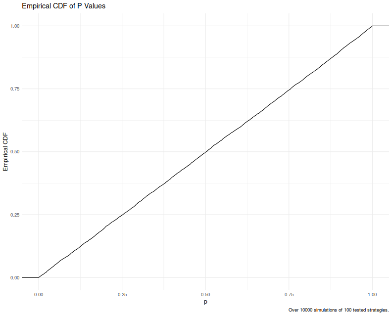
Let's confirm this empirically. We simulate the $\mu_i, x_i$ values, find the argmax of the $x_i$, and look at the associated $\mu_i$. Because this is a simulation we have access to the $\mu_i$. We compute what should be a standard normal $$ z = \frac{\mu_i - \left(\bar{x} + (1-\gamma)(x_i - \bar{x})\right)}{\sqrt{\frac{n-1}{n}\gamma\sigma_s^2 + \frac{1}{n}\sigma_l^2}}, $$ then compute the normal CDF of that thing. We plot the empirical CDF of the putative p-values. If our theory is correct this should look like the line segment from $(0,0)$ to $(1,1)$. In the plot below we see that indeed this is the case. I have tweaked the $n, \sigma_l^2, \sigma_s^2$ a few times and found that uniformity is not affected by these.
simit <- function(n, ss2, sl2=1.0, mu=5.0) {
    gamma <- sl2 / (sl2 + ss2)
    mu <- rnorm(n, mean=mu, sd=sqrt(ss2))
    x <- rnorm(n, mean=mu, sd=sqrt(sl2))
    xbar <- mean(x)
    iidx <- which.max(x)
    mui <- mu[iidx]
    xi <- x[iidx]
    nmu <- xi - gamma * (xi - xbar)
    nv2 <- (ss2*(n-1)*gamma/n) + (sl2/n)
    zval <- (mui - nmu) / sqrt(nv2)
    pval <- pnorm(zval)
    return(c(mui=mui, xi=xi, xbar=xbar, zval=zval, pval=pval))
}
nstrat <- 100
nsim <- 1e4
set.seed(1234)
blah <- replicate(nsim,simit(nstrat, ss2=0.3, sl2=0.2)) %>% t() %>% tibble::as_tibble()
library(ggplot2)
ph <- blah %>%
    ggplot(aes(x=pval)) +
    stat_ecdf() +
    labs(title='Empirical CDF of P Values',x='p',y='Empirical CDF',
         caption=paste0('Over ',nsim,' simulations of ',nstrat,' tested strategies.'))
print(ph)
I was initially surprised that this worked, because it seems like it would not deal properly with the selection pressure. On reflection, I think it is helpful to consider the two extremes of $\gamma$. When $\gamma=0$ we basically have spread in skill with no noise from luck. In that case we should observe that $\mu_i=x_i$. Our confidence bound becomes $$ \bar{x} + (x_i - \bar{x}) + z_{\alpha} \sqrt{\frac{1}{n}\sigma_l^2}, $$ but since $\sigma_l=0$ when $\gamma=0$, this is indeed just $x_i$. When $\gamma=1$ we have essentially no spread in skill and the noise of luck dominates. In this case all the $\mu_i$ are the same and equal to $\mu$, so we are better off estimating $\mu_i$ with $\bar{x}$, which has lower variance than $x_i$ alone (though technically $x_i$ contributes to $\bar{x}$). Our confidence bound becomes $$ \bar{x} + z_{\alpha} \sqrt{\frac{1}{n}\sigma_l^2}, $$ which just reflects the standard error around the sample mean, exactly as I would expect.
Compared to the DSR
In our previous blog post we performed a number of simulations on the DSR: spawn a population of true Sharpe ratios, simulate observed Sharpe ratios, select the strategy based on the in-sample Sharpe, compute the DSR, return the true Sharpe of the selected strategy and the DSR. Upon performing this simulation thousands of times we get some empirical estimate of how well the DSR performed. Here we will repeat those experiments, but consider our conditional estimator as well.
We simulate using some the values of some parameters from the original DSR paper. As in the original DSR paper, we assume 250 trading days per year, let $\sigma_s^2 + \sigma_l^2 = 0.5$ in "annualized units", let $T = 1250$ days (5 years at this cadence), assume returns are normally distributed, and fix $n = 100$. In addition to the DSR, we perform our conditional estimation, tuning it to conditionally test whether the true Sharpe is negative. To match the directional sense of the DSR we look at the upper tail CDF so that larger values mean the strategy is likely better; we will (conditionally) reject the hypothesis that the strategy is bad when our statistic is large, larger than $1 - \alpha$ for some threshold $\alpha$.
First the simulations. One oddity of note is that we set $\mu$ to be somewhat negative: If we set it to zero, there are few observed cases where the selected strategy is actually bad, and we have to infer the performance of these statistics based on a very small basis. Even with the value we set here, we actually selected a bad strategy in only approximately a quarter of the simulations.
exp_max_sr <- function(N) {
    mascher <- 0.5772156649
    (1 - mascher) * qnorm((1/N), lower.tail=FALSE) + mascher * qnorm(exp(-1)/N, lower.tail=FALSE)
}
dsr <- function(sr, T, N, Vsrs, Esrs=0, gamma3=0, gamma4=3, ...) {
    sr0 <- Esrs + sqrt(Vsrs) * exp_max_sr(N)
    serr <- sqrt((1 - gamma3 * sr + (gamma4 - 1)/4*sr**2) / (T-1))
    pnorm((sr - sr0) / serr, ...)
}
condest <- function(sr, srbar, n, ss2, sl2, test_snr=0, ...) {
  gamma <- sl2 / (sl2 + ss2)
  nmu <- sr - gamma * (sr - srbar)
  nv2 <- (ss2*(n-1)*gamma/n) + (sl2/n)
  return(pnorm(test_snr, mean=nmu, sd=sqrt(nv2), ...))
}
#' perform a number of simulations of normal skill plus normal luck,
#' compute the DSR on the results, return the SNR of the strategy
#' selected for having maximal sharpe, along with that maximal sharpe and the DSR statistic.
#' also compute the conditional threshold.
sim_machine <- function(T, n, sigmasq_tot, mu=0, nsims=100000, dpy=250) {
  require(tibble,quietly=TRUE)
  sigma_luck_day <- sqrt(1/T)
  sigma_tot_day <- sqrt(sigmasq_tot / dpy)
  sigma_skill_day <- sqrt(sigma_tot_day^2 - sigma_luck_day^2)

  simvals <- replicate(nsims, {
    skills <- rnorm(n, mean=mu, sd=sigma_skill_day)
    srs <- rnorm(length(skills), mean=skills, sd=sigma_luck_day)
    maxsr <- max(srs)
    nidx <- which.max(srs)
    selskill <- skills[nidx]
    dsrv <- dsr(maxsr, T, N=n, Vsrs=sigma_tot_day^2)
    srbar <- mean(srs)
    condp <- condest(maxsr, srbar, n=n, ss2=sigma_skill_day^2, sl2=sigma_luck_day^2, test_snr=0, lower.tail=FALSE)
    c(skill=selskill, dsr=dsrv, maxsr=maxsr, condp=condp)
  })
  tibble::as_tibble(t(simvals))
}

T <- 1250
n <- 100
sigmasq_tot <- 0.5
set.seed(1234)
results <- sim_machine(T=T, n=n, sigmasq_tot=sigmasq_tot, mu=-0.05, nsims=5e6)
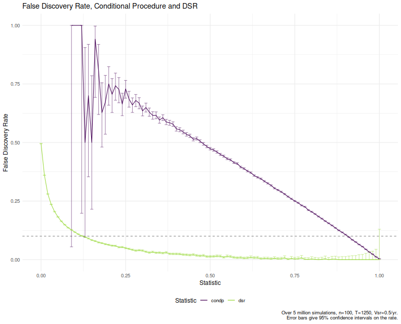
Now we analyze the results. Because our conditional procedure is, well, conditional, we will not look at these from the usual frequentist lens of type I and type II error rates. Instead we will condition on the statistic taking a certain value, then compute the proportion of the time the selected strategy is bad (i.e. has a negative population Sharpe ratio). We expect that when our statistic is large, the number of such "False Discoveries" should be low. In fact we would like that the false discovery rate is one minus our conditional statistic. (Recall we flipped the sign so more is better, to match DSR.)
Here is that plot for the 5 million simulations. We plot a horizontal line at 0.10. From this plot it would seem that to achieve a 10% FDR using the DSR we would have to accept a strategy (reject the null) whenever DSR is bigger than around 0.125. For the conditional procedure the value appears to be just around 0.90, as we would expect.
From this plot we see that the conditional procedure approximately controls the False Discovery Rate, at least for small FDR rates. That is, if you wanted to ensure your FDR was below 5 percent, say, you would require the conditional procedure to produce a value of 0.95 before trading. It is not clear to me why the line here deviates from the $y=1-x$ line at all. In contrast to the simulations above, I suspect that the issue is that the "p value" of the conditional procedure is not independent of the statistic's value, and that causes the procedure to be somewhat conservative. Compared to the DSR, however, this is a second order problem.
compute_rejrates <- function(stacked_results, conf.level=0.95, dsr_thresh=0.95) {
  stacked_results %>%
    group_by(stat_group, stat) %>%
      summarize(`Bad Strategy`=sum(skill < 0), Total=n()) %>%
    ungroup() %>%
    mutate(`False Discovery`=`Bad Strategy` / Total) %>%
    mutate(conf.lo=mapply(function(x, n)  {prop.test(x, n, conf.level=conf.level)$conf.int[1]}, `Bad Strategy`, Total)) %>%
    mutate(conf.hi=mapply(function(x, n)  {prop.test(x, n, conf.level=conf.level)$conf.int[2]}, `Bad Strategy`, Total))
}
bind_rows(condp=results %>%
    mutate(stat_group=round(condp, 2)),
  dsr=results %>%
    mutate(stat_group=round(dsr, 2)),.id='stat') %>%
  compute_rejrates() %>%
  ggplot(aes(stat_group,`False Discovery`,group=stat,color=stat)) +
  geom_errorbar(aes(ymin=conf.lo,ymax=conf.hi),alpha=0.5) +
  geom_line() +
  geom_hline(yintercept=0.10,linetype='dashed',alpha=0.5) +
  labs(x='Statistic',y='False Discovery Rate',
       title='False Discovery Rate, Conditional Procedure and DSR',
       color='Statistic',
       caption='Over 5 million simulations, n=100, T=1250, Vsr=0.5/yr.\nError bars give 95% confidence intervals on the rate.')
Summary
We crafted a conditional test statistic that, conditional on observing the maximum and mean of the in-sample Sharpe ratios, is approximately uniformly distributed when the true Sharpe of the selected strategy is zero. In contrast to the DSR, which is wildly miscalibrated, it approximately controls for the False Discovery Rate: if you wish to have a False Discovery Rate less than $\beta$, you should only trade a strategy when this statistic is greater than $1-\beta$. Our statistic only requires the max and mean Sharpe, the number of strategies and the variance of the skill and the luck. I believe the procedure can be adapted to the case of general correlation structure on the noise.
This could have been a blog post
An interesting fact about our conditional procedure is that it does not rely at all on the asymptotic maximum of the normal distribution, the so-called "False Strategy Theorem" that López de Prado has been flogging in four-plus papers. Instead it seems to smooth between the two extremes of all-luck and all-skill cases, matching our intuition for both of those, using the sample mean and maximum. The reason this is just a blog post and not four papers is not just because the derivation took me less than an hour, but mostly because I don't think the problem setup is a good match for reality. As I complained in the previous blog post, the assumption that skill is normally distributed is a poor match for reality in my view. Moreover, I would expect that strategies are parametrized by some knobs which control both their population Sharpe and how correlated their backtests are, while the setup to this problem ignores that altogether.
References
- Bailey, David H. and López de Prado, Marcos. 2014. The Deflated Sharpe Ratio: Correcting for Selection Bias, Backtest Overfitting and Non-Normality Journal of Portfolio Management, 40(5): 94-107. (40th Anniversary Special Issue), DOI: 10.2139/ssrn.2460551
- Arnold, B. C., Balakrishnan, N. and Nagaraja, H. N. 2008. A First Course in Order Statistics, SIAM.
- Kaufmann, E. and Reiss, R.-D. 1992. On conditional distributions of nearest neighbors Journal of Multivariate Analysis, 42(1): 67-76.